Example: Imposed electric and magnetic fields
This article explains how to model the effect of an external, quasi-static electric field \(\overrightarrow E\) on a spatially-detailed neuron model. The field is assumed to be perfectly imposed outside the neuron, as is the case for high-intensity fields and high-conductivity surrounding media (such as a lonely neuron on a dish, or whenever the effects of the surroundings can be just simplified away without much loss).
First of all, let’s install the required software, if on certain platforms like Colab that run the bare notebooks:
import os; from pathlib import Path
if 'COLAB_BACKEND_VERSION' in os.environ:
!TMP=$(mktemp -d); git clone https://eden-simulator.org/repo --depth 1 -b development "$TMP"; cp -r "$TMP/." .; rm -rf "$TMP"
exec(Path('.binder/install_livenb.py').read_text())
if 'DEEPNOTE_PROJECT_ID' in os.environ: exec(Path('../.binder/install_livenb.py').read_text())
Get a cell model
For example, from Mainen et al. 1995:
# Download and unpack
import urllib.request; from zipfile import ZipFile
urllib.request.urlretrieve('https://codeload.github.com/OpenSourceBrain/MainenEtAl_PyramidalCell/zip/refs/heads/master', 'Mainen95.zip')
with ZipFile('Mainen95.zip', 'r') as zipp: zipp.extractall()
nml_dir = 'MainenEtAl_PyramidalCell-master/neuroConstruct/generatedNeuroML2/'
cell_filename = nml_dir+"MainenNeuroML.cell.nml"
And analyse it with EDEN:
celltype_name = 'MainenNeuroML'
import eden_simulator
cells_info = eden_simulator.experimental.explain_cell(cell_filename)
cell_info = cells_info[celltype_name]
comp_mid_seg = cell_info['comp_midpoint_segment']
n_comps = len(comp_mid_seg)
print(f'Compartments: {n_comps}')
xyz = cell_info['comp_midpoint'].T # break down by coordinate
Compartments: 739
Prepare to run simulations
We’ll re-use the following code for a single-neuron model to apply the equivalent \(I_{ext}\) of the imposed field (as seen in the following), and record and display the resulting \(V_m\), over all parts of the neuron.
cell_pop_name = 'Pop'
tabline = '\n '
comp_locators = eden_simulator.experimental.GetLemsLocatorsForCell(cell_info)
cell_voltage_paths = [ f'{cell_pop_name}[0]/{loc}/v' for loc in comp_locators ]
def MakeNmlModel(model_name, cell_info, Iext_nA, pulse_sec):
assert(pulse_sec[1]>pulse_sec[0])
model_file = f'''<neuroml>
<include href="{cell_filename}"/>
<pulseGenerator id="pulseNamp" delay="{pulse_sec[0]} s" duration="{pulse_sec[1] - pulse_sec[0]} s" amplitude="1 nA"/>
<network id="Net_{model_name}">
<population id="{cell_pop_name}" component="{celltype_name}" size="1" />
<inputList id="ElectrodeStim" component="pulseNamp" population="{cell_pop_name}">
{tabline.join([ f'<inputW id="{comp}" target="{cell_pop_name}[0]" weight="{curr}"'
+f' segmentId="{cell_info["comp_midpoint_segment"][comp]}"'
+f' fractionAlong="{cell_info["comp_midpoint_fractionAlong"][comp]}" destination="synapses"/>'
for comp, curr in enumerate(Iext_nA)])}
</inputList>
</network>
</neuroml>'''
with open(f'Net_{model_name}.nml', 'wt') as f: f.write(model_file)
def MakeNmlSimFile(model_name, sim_duration_sec):
tabline = '\n '
sampling_period_sec = 0.1e-3
sim_file = f'''<Lems>
<Include href="Net_{model_name}.nml"/>
<Simulation id="MySim" length="{sim_duration_sec} sec" step="10 usec" target="Net_{model_name}">
<EdenOutputFile id="OutFile" href="file://Results_{model_name}.gen.txt" format="ascii_v0" sampling_interval="{sampling_period_sec} s">
{tabline.join([ f'<OutputColumn id="v_{loc}" quantity= "{path}" output_units="V"/>' for loc, path in zip(comp_locators, cell_voltage_paths)])}
</EdenOutputFile>
</Simulation>
<Target component="MySim"/></Lems>'''
sim_filename = f'LEMS_Sim_{model_name}.xml'
with open(sim_filename, 'wt') as f: f.write(sim_file)
return sim_filename
Since we’ll be doing physics with the simulation’s results, let’s add physical units with pint.
#!pip install -q pint
def ResultsToVm(results):
import numpy as np
from pint.registry import Quantity as Q
neuron_membrane_voltage = np.array([results[path] for path in cell_voltage_paths])
neuron_membrane_voltage = Q(neuron_membrane_voltage,'V')
return neuron_membrane_voltage
Let’s make a 2D plot of \(V_m\) per compartment:
def ShowVmRaster(neuron_membrane_voltage):
from matplotlib import pyplot as plt
im = plt.imshow(neuron_membrane_voltage.m_as('mV'),
extent=[ *rec_time_axis_sec[[0,-1]], n_comps, 0 ],
aspect='auto', interpolation='none', cmap ="viridis")
cbar = plt.colorbar(im); cbar.set_label('Voltage (mV)')
plt.ylabel('Compartment #'); plt.xlabel('Time (sec)');
And cool 3D animations in general:
import numpy as np; import k3d; from eden_simulator.display.animation import subsample_trajectories
def TimeLabel(anim_axis,sampled_time):
k3d_label_dict = { str(real_time): f't = {sim_time*1000:.1f} ~ ms' for (real_time, sim_time) in zip(anim_axis, sampled_time) }
return k3d.text2d(k3d_label_dict, (0.,0.))
animation_speed=0.0048
def makeplot(cell_info, values, rec_time_axis_sec, color_range=[-70, -20], color_map='rainbow', plot=None):
from eden_simulator.display.animation import subsample_trajectories
samples_vm, anim_axis, sampled_time, (sampled_voltage,) = subsample_trajectories(
rec_time_axis_sec, [neuron_membrane_voltage.m_as('mV').T], animation_speed=animation_speed, animation_frames_per_second=24)
plot = Plot()
plot += plot_neuron(cell_info, sampled_voltage, time_axis_sec=anim_axis,
color_range=color_range, color_map=color_map);
plot.camera = plot.get_auto_camera(pitch=30, yaw=10)[:6]+[0,1,0] # set 'y' to up ! vecs are pos, tgt, up
plot += TimeLabel(anim_axis,sampled_time) # add 2d elements AFTER setting auto camera
return plot, (anim_axis, sampled_time)
def PointUp(plot):
plot.camera = plot.get_auto_camera(pitch=30, yaw=10)[:6]+[0,1,0] # set 'y' to up ! vecs are pos, tgt, up
Now, to the experiment.
Physics
Let’s introduce some electro-physical terms and laws that will help understand the following (or skip them if they’re well known):
A vector is, for the purposes of this topic and Euclidean space, a “longer” or “shorter”, generally directional property drawn as an arrow. Arrows of “zero” length that are ineffectual and directionless can exist, we just don’t draw them. As mathematical symbols we write vectors down as lower-case names e.g. \(r\) but either with an arrow on top \(\overrightarrow{r}\), or in boldface \(\mathbf{r}\).
For instance: Points in space can be expressed as arrows from an arbitrary point of reference or origin, to them. Velocity \(\mathbf{v}\) can be expressed as its direction, with length in corresponding units of measure.
If we (very conveniently) break down a vector to our three accessible dimensions or axes of movement (i.e. left-right, up-down and front-back), we can break it down into \(x, y, z\) components parallel to each dimension. We can then name unit vectors \(\mathbf{\hat x}, \mathbf{\hat y}, \mathbf{\hat z}\) for the associated dimensions, and express \(x, y, z\) as real numbers, that represent multiples of the aforementioned unit vectors. Thus \(\forall~\mathbf{r}~\exists~x, y, z \in \mathbb{R}^3 : \mathbf{r} = x \mathbf{\hat x} + y \mathbf{\hat y} + z \mathbf{\hat z}\).
A field \(\overrightarrow{F}(\overrightarrow{r})\) is a mathematical function that maps locations to vectors. We generally use capital letters to name those, to avoid confusion. Fields can represent directional attributes (of e.g. physical phenomena) that exist over places. For every location, there is one particular vector; we draw a few of them to get a rough picture. An easy to understand example of a field is the velocity of a flock, crowd or stampede of animals; nearby animals have about the same velocity lest they bump on each other.
Electrically conductive materials such as the intracellular (and normally extracellular) environment are full of freely moving charges (of electrons, ions and such). These charges are pushed around by an electric force field \(\overrightarrow{E}\); its force \(\overrightarrow{F}\) is amount of electric charge \(q\) times the field’s intensity. We can write this down as \(\overrightarrow{F} = q \overrightarrow{E}\); the field is hence measured in Newtons over Coulombs. (Another better known force field is gravity acting likewise on mass; we just have never observed negative mass.) Within neurons, this field is caused by the electric charge of the membrane (on both sides) and relative differences thereof over space and time. But in this chapter, we’ll also add the influence of external fields to the mix.
Movement through a force field imparts or deducts kinetic energy \(K\); movement of a positive charge in the direction of the electric field imparts, movement in the opposite direction deduces, movement sideways does neither. This all is proportional to charge amount and field intensity, and reversed for negative charges (and zeroed for zero charges, field, movement). We can write that down as \({d K} = q \overrightarrow{E} \cdot d\mathbf{r}\) for small movements \(d\mathbf{r}\) (remember that \(\mathbf{E}(\mathbf{r})\) changes with \(\mathbf{r}\)). We can then define the energy per charge gained along a certain path \(L\) as the \(\frac{\Delta Κ}{q} = \int_L \overrightarrow{E} \cdot d \textbf{r}\). This is what we call the electric tension or voltage along a path! Volts = Energy (Joules) over Charge (Coulombs). Considering that Energy is Force times Length, we also measure \(\overrightarrow{E}\) more commonly in Volts over Metres. Note that the opposite voltage applies over the same path in the opposite direction.
In some cases, it doesn’t matter which path a particle makes to move from \(\mathbf{a}\) to \(\mathbf{b}\); they all will impart the same energy per charge. Then we can define a scalar electric potential \(U(\textbf{r})\) or \(U(x,y,z)\) which represents the voltage between locations and some arbitrary point of reference. Keep in mind that the potential decreases in value along the lines of the field! The point of reference doesn’t really matter because we should only consider the difference from point to point, much like with integrals. Note that the effect of such fields or their “potentials” can be summed linearly when they are present together, as long as they don’t interfere with each other (significantly).
In other cases, the path does matter, which complicates things. In fact, a charged particle could get more and more energy by following two different paths from \(\mathbf{a}\) to \(\mathbf{b}\), one forwards than one backwards in an endless loop! This happens when we’re dealing with a time-varying magnetic field and the electro-magnetic induction that it causes. In such cases, we can’t define an unambiguous \(U(x,y,z)\) over space, we’ll just have to trace the path being taken. Remember that the charges’ path is constrained by the conductors they can pass through, and otherwise driven by the forces applied on them, that can’t just go however they please. Hence there is a well defined voltage between two points, along a certain path. But when, say, a wire does go in loops it can accumulate voltage multiple times over (roughly) the same path.
Even when the path does matter, this doesn’t mean that “membrane voltage” and other are meaningless. They remain part of the total field and energy differential, we just add the effect of the field’s rotational component on top. The part with a “potential” is due to distributions of electric charge (for instance, between the cell membrane’s sides) and the rotational part is due to a changing magnetic field, as per Maxwell’s equations.
The actual quantity charge moving because of the applied forces is usually determined by Ohm’s law: the more conductive the material is the more the charges move. We can have an electric field even when nothing moves, observe an unplugged mains socket. As the socket gets plugged sparks may fly because as the conductors get to touch, the difference in potential is across a smaller and smaller distance before it is “moved” to the load after the plug.
Classic cable equation
Having said all that, we can apply fields on neurons as follows.
Neural cable theory assumes for each compartment of a neuron:
two electric nodes, one for inside the membrane and one for outside the membrane. The voltage between them is \(V_m = U_{int} - U_{ext}\);
membrane capacitance between these nodes, and a bunch of trans-membrane channels with reversal-potentials (which can be lumped into a Thévenin equivalent);
axial resistance between the inner nodes of adjacent compartments. \(I_{a,ij} = \frac{U_{int,i} - U_{int, j}}{R_{a,ij}}\)
Now, the simplest model (shown here) assumes that the exterior side of all compartments shares the same potential i.e. the outside of the cell is all shorted together. Hence \(U_{int,i} - U_{int, j} = V_{m,i} - V_{m,j}\). That could be true in the case of an isolated neuron with highly-conductive, non-polarised surroundings. In practice, more interesting things can also happen.
In the more general case, we can consider voltages \(V_{ext, ij}\) between each pair \(i,j\) of adjacent compartments. Keep in mind that these do not matter locally across a membrane; if the exterior of a compartment is at a certain potential then the interior side will only differ by \(V_m\) regardless. Thus the effect of external voltage differences only appears as voltage gradients from compartment to compartment. Mathematically, this means that from the whole cable equation, only the axial current equation has to include the change $U_{int,i} - U_{int, j} $ $= (V_{m,i} + U_{ext,i}) - (V_{m,j} + U_{ext,j}) $ \(= (V_{m,i} - V_{m,j}) + (U_{ext,i} - U_{ext,j})\) \(= V_{m,ij} + V_{ext,ij}\). Thus axial current between two adjacent compartments is the difference in their \(V_m\) divided by axial resistance, plus the voltage between their exteriors divided by the same.
Since they are not part of the NeuroML specification, EDEN doesn’t offer a way to directly specify extracellular electric fields; the current assumption is that \(U_{ext}\) is the same everywhere. Nonetheless, fields can be modelled accurately by modelling the equivalent current flows that they cause inside the neuron, as explained above. We can do this in our NeuroML model by injecting in each compartment \(i\), a pseudo-current that is the algebraic sum of all equivalent flows from this compartment to adjacent ones, caused by external voltages: \(\displaystyle I_{eq,i} = \sum_j{ {V_{ext,ji}} \over R_{a,ij}}\). In linear algebra terms, \(\mathbf{I}_{eq} = \mathbf{G} \mathbf{U}_{ext}\) where \(\mathbf{G}\) is the conductance matrix between adjacent compartments. This technique is also presented in McNeal (1976) and related literature.
Observe that the total pseudo-current injected to the neuron is zero. At the same time, do note that the real current flowing through a neuron because of the field is accounted for; as alterations in conductance-based trans-membrane current, that follow the applied voltage gradient from one cell to the other. For instance, a resting cell slightly polarised from side to side will have differential changes in resting potential, and thereby differential leak current.
def GetAxialConductanceMatrix(cell_info):
'''Form the axial resistance matrix $I_a = G*V$ connecting compartments.
Parameters
---
cell_info : dict[str, object]
The cell information retrieved by :py:`eden_simulator.experimental.explain_cell`.
Returns
---
m : scipy.sparse.sparray
A sparse symmetric matrix of inter-compartment conductance, in the same units as `cell_info['comp_conductance_to_parent']`.
TODO
'''
comp_ga = cell_info['comp_conductance_to_parent']
iii = []; jjj = []; vvv = [] # Construct the lists (i,j,v)
for i,p in enumerate(cell_info['comp_parent']):
g = comp_ga[i]
if p >= 0:
iii += [ i, p, i, p] # add 4 sparse elms in one go
jjj += [ p, i, i, p]
vvv += [+g,+g,-g,-g] # same as:
# G[i,p] += g
# G[p,i] += g
# G[i,i] -= g
# G[p,p] -= g
import scipy
G = scipy.sparse.coo_matrix((vvv,(iii,jjj))).tocsr() # needs csr for some reason
return G
G_nS = GetAxialConductanceMatrix(cell_info)
Steady field shape
If the field varies spatially only in magnitude (its “pulse shape” remains the same, so to speak), we need to apply the above calculations just once for arbitrary units, to find the relative weights. Then at simulation time, we can vary the amplitude of all pseudo-current injection points by this weight factor.
Tip: Such simulations can be modelled in pure NeuroML, without any EDEN-specific extensions - albeit with the help of explain_cell to tell us where the actual compartments are located in the neuron model and how they are electrically linked.
Uniform electric field
Let’s say the electric field of amplitude \(a\) points to the \(+y\) axis: \(\overrightarrow{E} = a \, \hat{y} ~~ \frac{V}{m}\). Then we can define an electric potential \(U(x,y,z) = -a y\) all over the place. Note that as long as we care about the difference i.e. voltage, we can assume the point where \(U = 0\) wherever (in this case where \(y = 0\) for simplicity).
def ElectricPotential_Uniform(x,y,z):
"Get the extracellular potential for a uniform field of 1 V/m in volts for x,y,z in microns."
return -y * 1 * 1e-6 # 1 μV/μm
Vext_V = 50 * ElectricPotential_Uniform(*xyz) # let's say 50 V/m or mV/mm
Iext_nA = G_nS @ Vext_V # nS * V
Let’s look at the pseudo-currents we’re about to inject in each compartment, to apply the externally imposed field.
import k3d; from eden_simulator.display.spatial.k3d import Plot, plot_neuron
Im_uniform_plot = plot = Plot()
plot += plot_neuron(cell_info, Iext_nA*1e3, color_map='bwr', color_range=[-10, +10]);
PointUp(plot); plot.show_html()
Plot the following graph at different scales of magnitude, to appreciate the equivalent currents in both the thick and the thin compartments.
One may be surprised to see that adjacent compartments along a straight line have a non-zero injected current! How can this be true, surely all currents add up to zero‽ Well, the equation is pretty clear about it: The quantities \(\frac{V{i-1}-V_i}{R_{i-1,i}}\) and \(\frac{V_i-V_{i+1}}{R_{i,i+1}}\) are, in any way, unequal. In fact the only place where injected current is precisely zero along the field’s direction, is between electrically identical compartments on the model’s stylized axon (between the nodes of Ranvier).
Well then, how exactly does it make sense that the current balance in an intermadiate compartment would be nonzero? where would it draw the current from‽ Remember, we are calculating a shift in axial currents here. If the shift indicates a divergence in the flow of current, this simply means that ceteris paribus the compartment has more or less of a \(V_m\) than its surroundings. Which is also what with an external point electrode, or in our case, when the neurites curve in the direction of the field and then back against it.
Let’s run the simulation now:
model_name = 'ImposedField_Simple'; pulse_sec = [0.005,0.040]
MakeNmlModel(model_name, cell_info, Iext_nA, pulse_sec=pulse_sec)
sim_filename = MakeNmlSimFile(model_name, sim_duration_sec=0.1)
results = eden_simulator.runEden(sim_filename)
rec_time_axis_sec = results['t']; neuron_membrane_voltage = ResultsToVm(results)
And see what happened:
# Add a cute arrow to the uniform field's direction
def ArrowMesh(p0,p1,stem_radius=5,tip_radius=10,tip_length=20):
d = np.array(p1) - p0
import trimesh
cone = trimesh.creation.cone(radius=tip_radius, height=tip_length,transform=trimesh.geometry.align_vectors([0, 0, 1], d))
tube = trimesh.creation.cylinder(radius=stem_radius, segment=[p0,p1])
return k3d.mesh(np.r_[cone.vertices+p1, tube.vertices].astype('float32'), np.r_[cone.faces,len(cone.vertices)+tube.faces].astype('uint32'), color=0xffc700)
def ColorByPulse(anim_axis,sampled_time,on_off,colors):
return { str(real_time): (colors[1] if on_off[0] < sim_time < on_off[1] else colors[0] ) for (real_time, sim_time) in zip(anim_axis, sampled_time) }
Vm_uniform_plot,_ = plot,(anim_axis,sampled_time) = makeplot(cell_info, neuron_membrane_voltage, rec_time_axis_sec, color_range = [-80,-20])
arrow = ArrowMesh([50,-50,0], [50,+100,0])
arrow.color = ColorByPulse(anim_axis, sampled_time, pulse_sec, [0xc0c0c0,0xffc700])
# arrow.color = { f'{(5e-3)/animation_speed-.001}': 0xc0c0c0, f'{(5e-3)/animation_speed}': 0xffc700, f'{(205e-3)/animation_speed-.001}': 0xffc700, f'{(205e-3)/animation_speed}': 0xc0c0c0, }
plot += arrow
plot += k3d.text('\\overrightarrow{E}',position=[50, 120, 0], label_box=False, reference_point='cb', size=2, color=0xffb700)
plot.show_html()
Try the opposite field. What happens? When and where did the neuron fire first this time and why? Now try the original field but applied for 30 msec (pulse_sec = [0.005, 0.040]), and watch again. How did this happen?
Having shown how a strong enough electric field can itself make a neuron fire, in the following simulations we will use weaker sub-threshold fields to just show the spatial polarisation of the neuron.
Disc electrode
Now, let’s simulate the effect of a flat disc electrode. The electric potential it induces follows the formula:
where \(a\) is the radius of the electrode and \(r, z\) are the distances parallel and perpendicular to the disc, and with \(U = 0\) far far away. From Wiley and Webster (1982).
import numpy as np
def ElectricPotential_ConductiveDisc(x,y,z, middle, radius):
"Get the relative extracellular potential for a disc electrode on the x-z plane field, for x,y,z in microns."
x,y,z = x - middle[0], y - middle[1], z - middle[2]
a = radius; norm = np.linalg.norm
r = norm([x,z], axis=0);
return (2/np.pi)*np.arcsin(2*a/(norm([r-a,y], axis=0) + norm([r+a,y], axis=0)))
disc_middle = np.array([-162.88156, -150, -4.9890413]); disc_radius = 50
Vext_V = 0.02 * ElectricPotential_ConductiveDisc(*xyz, disc_middle, disc_radius)
# plt.plot(Vext_V)
Iext_nA = G_nS @ Vext_V # nS * V
This time, we apply a localised field, with the electrode at a potential \(+20~mV\). It is prudent to visualise the electrode’s location and computed potential, to fix mistakes at this stage before interpreting the simulation’s results.
from matplotlib import pyplot as plt
image_size_microns = [200,400]; imgsiz = image_size_microns
X,Y = np.meshgrid(np.arange(0,imgsiz[0])+disc_middle[0],np.arange(0,imgsiz[1])+disc_middle[1]); Z = 0*X+disc_middle[2]
sampUext = 0.02*ElectricPotential_ConductiveDisc(X,Y,Z,disc_middle, disc_radius)
dpi = 144
fig,ax = plt.subplots(figsize=[2*imgsiz[0]/dpi,2*imgsiz[1]/dpi],dpi=dpi)
ax.pcolormesh(X,Y,sampUext,cmap='Reds')
CS = ax.contour(X, Y, sampUext*1e3,linewidths=1); ax.clabel(CS, fontsize=8)
ax.set_axis_off();ax.axis('equal')
fig.subplots_adjust(top=1.0, bottom=0, right=1.0, left=0, hspace=0, wspace=0)
fig.savefig('uext_disc.png', bbox_inches='tight', pad_inches=0)
fig.dpi=fig.dpi/2 # just for publishing this big vertical image...
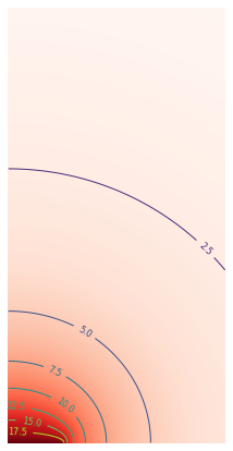
To illustrate the effect, the proximity and tininess of the electrode have been exaggerated. Please also disregard for a moment that the artificial axon goes through the electrode, it won’t affect the result.
def AddBillboardXY(filename,off,ext,name=None):
return k3d.mesh(
vertices=[off+[ 0, 0,0],off+[ext[0], 0,0],
off+[ext[0],ext[1],0],off+[ 0,ext[1],0]],
indices=[[0,1,2,],[2,3,0]],uvs=[[0,1],[1,1],[1,0],[0,0]],
side='double',
texture=open(filename,'rb').read(),
texture_file_format=filename.split('.')[-1],
color=0xffffff,name=name)
def DiscMesh():
import pyvista as pv
import logging; k3d.helpers.logger.setLevel(logging.WARN) # silence whine for float64 numbers
mesh = pv.Cylinder(center=disc_middle, direction=[0, 1, 0], radius=disc_radius, height=1);
return k3d.vtk_poly_data(mesh, color=0xc6884b);
Uext_disc_plot = plot = Plot()
plot += plot_neuron(cell_info, Vext_V*1e3,color_range=None, color_map='reds');
# Add a graph of the field
graph = AddBillboardXY('uext_disc.png',disc_middle,imgsiz,name='Field graph')
graph.opacity = 0.75; plot += graph
plot += DiscMesh() # Add the electrode
PointUp(plot); plot.show_html()
Looks good, let’s run the simulation then.
model_name = 'ImposedField_Disc'; pulse_sec = [0.005,0.035]
MakeNmlModel(model_name, cell_info, Iext_nA, pulse_sec=pulse_sec)
sim_filename = MakeNmlSimFile(model_name, sim_duration_sec = 0.050)
results = eden_simulator.runEden(sim_filename)
rec_time_axis_sec = results['t']; neuron_membrane_voltage = ResultsToVm(results)
plt.figure(figsize=[9,4]);ShowVmRaster(neuron_membrane_voltage); #plt.clim([-70, -67.5])
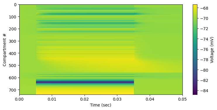
The cell has been slightly polarised but not past rheobase. Note that the shift in charges completed in some 16 msec, but even faster for most parts. Let’s see how that looks in 3-D:
Vm_disc_plot,_ = plot,(anim_axis,sampled_time) = makeplot(cell_info, neuron_membrane_voltage, rec_time_axis_sec, color_range = [-70,-67.5])
plate = DiscMesh()
plate.color = ColorByPulse(anim_axis,sampled_time,pulse_sec,[0xc6884b,0xff0000])
plot += plate
plot.show_html()
Magnetic field by a coil
More physics
Note: The following analysis is called quasi-static since it neglects EM wave dynamics. If radio-frequency effects are is significant, well … perhaps a timestep in the order of μsec is too big, and this level of modelling too coarse to be honest. Or the effect could be lumped at this level, with an empirical formula.
When a magnetic field changes, it induces a curl on the electrical field: \(\nabla \times \mathbf{E} = -\frac{\partial \mathbf{B}}{\partial t}\) . The electric potential is then ill defined, because one could go from point A to point B following however many loops and gain an arbitrary amount of energy. However! The potential through a conductor (neural cable) is still well defined, and so is the the induced electromotive force i.e. the line integral of the field, from compartment A to compartment B. Which we can calculate just fine, we’ll just have to (in theory) trace the exact path taken. If the compartments are chopped finely enough and the field is smooth enough, we can sample the field at the midpoints \(x_i\) of the compartments only, and approximate \(V_{ij} \approx - \Delta\overrightarrow{x}_{ij} \cdot \frac{1}{2} (\vec E(x_i)+\vec Ε(x_j))\) .
An example about it will be provided on popular demand. The interested reader is kindly requested to contact us with an use case to make us go faster.
General time-varying field
In the more general case where the shape of the field does change over time, the virtual currents also need to be re-sampled along the time axis as well; hence, we need to feed each pseudo-source with an arbitrary waveform. EDEN can easily handle this through its NeuroML extension for input time series.
Magnetic field by a moving coil
An example about it will be provided on popular demand. The interested reader is kindly requested to contact us with an use case to make us go faster.
Further considerations
Since cells are laid out as simple trees rather than coils, we don’t expect to see too drastic effects over just one neuron; consider the coupling between neurons at the tissue scale. In this case, besides the electric synapses obviously connecting adjacent cells, modellers have to consider more indirect (but at scale, significant) paths to electric coupling.
When simulating multiple neurons, or when the field’s coordinates are different from the neuron’s origin: Remember to translate/rotate by the neuron’s pose!
Feature size of the neurons and the fields
An important property of the field is its “feature size”, or the smallest distance over which it may change significantly. For a good approximation of the field, sampling at points must be at least as fine-detailed as the field is in the vicinity.
If the (radius of) curvature of the field is tighter than the distance between compartments, don’t just sample the midpoints; consider the whole path through the morphology’s
<segment>s, with a tool like LFPykit. On the other hand, in this case the compartments should be fine enough that local effects are fully captured. Which brings us to …If the morphology’s segments are too coarse … well, get a better morphology, or somehow simulate a more “likely” one. For instance, if some segments are stylised and unrealistically long, subdivide them and add some realistic curvature as applicable.
Be especially wary of the neuron’s axons: modellers often simplify them to huge straight sticks, which then catch a disproportionate lot of induced field and hence apply a very large and very wrong influence on the cell’s behaviour. As a great mind once put it, if something is a fiction and it drives the cell, then the cell is driven by a fiction.
Detail of the surroundings
In the above we assumed a linear, uniform, isotropic, totally dull extracellular environment. But the real tissue may have anatomical features which constrain electrical flow, the dura just to name one. Be aware and creative while negotiating brain effects, and contact us if you have questions. If the effect is really local, it might make sense to constrain simulation to that point and crank up the resolution (see also other finite-element and molecule-based programs).
Ephaptic coupling
Sometimes instead of a blunt and unnaturally powerful electrode, we want to model the interactions between cells (with less power to give and more ‘internal resistance’ so to speak). In the finer-detailed case, there are lots of compartment-compartment interactions: to maintain numerical stability, the whole tissue gets coupled into a huge linearised system that we’d have to solve on each timestep(!). Simulators like ELFENN try to take care of this but can handle a limited number of compartments; we are also developing an EDEN-beased solution even for this tricky subject, stay tuned.
There are other cases though, such as within certain axon bundles, where we can see the potentials flowing in a synchronised wave; we can then assume this stampede immovable by any one neuron, and study the dynamics of that one neuron as forced by the imposed neural wave around it. As seen in this article.
Related resources
Many relevant discussions and pitfalls to watch out for can be found on the NEURON forum. Search for “extracellular”, “field” or so.
For NEURON users: This is the
stimpart of the popular extracellular_stim_and_rec scripts.