



Tutorial: A network of detailed cells
This tutorial shows how to build an active network of detailed neurons, simulate it to get the neurons’ potentials over time in full spatial detail, and display these data as an animated 3D display.
Refer also to the previous introductory articles for the basics of NeuroML and spatially detailed cells.
First of all, let’s install the required software, if on certain platforms like Colab that run the bare notebooks:
import os; from pathlib import Path
if 'COLAB_BACKEND_VERSION' in os.environ:
  !TMP=$(mktemp -d); git clone https://eden-simulator.org/repo --depth 1 -b development "$TMP"; cp -r "$TMP/." .; rm -rf "$TMP"
  exec(Path('.binder/install_livenb.py').read_text())
if 'DEEPNOTE_PROJECT_ID' in os.environ: exec(Path('../.binder/install_livenb.py').read_text())
import numpy as np
import matplotlib as mpl
import matplotlib.pyplot as plt
Constructing the network
Building a network model generally involves the following actions:
place the cells forming the network;
connect the cells with synapses;
add the experimental rig: add external stimuli and probe the electro-chemical variables of interest.
Placing neurons
First, let’s decide where to place the neurons in the model. For this tutorial, assume that neurons are uniformly spread over, say a tall cylinder that stands for a microcolumn. We’ll use an evenly spread quasi-pseudo-random distribution, which won’t randomly form misleading clumps like a true random sample would. We’ll also sort the cells by distance along the cylinder, to give more meaning to the the resulting rasters and correlation matrices.
Check the following code also for a neat way to get uniformly random points over an arbitrary shape:
check they fall on the shape, keep only those who do.
resample to fill in the remaining slots.
Kind of like painting with a stencil :)
!pip install -q 'scipy>=1.12' # for an evenly spread, *quasi* pseudo random distribution
# get a few cells
# randomize x, y, z using e.g. a cylinder
# https://docs.scipy.org/doc/scipy/reference/generated/scipy.stats.qmc.Halton.html#scipy.stats.qmc.Halton
seed = 123
N_cells = 30
# Points will be placed in a cylinder of given radius and height
region_radius = 50 # microns
region_height = 200

from scipy.stats import qmc
position_rng = qmc.Halton(d=3, scramble=True, seed=seed)

# Use rejection, to make the 3D points conform to an arbitrary domain
remaining_cells = N_cells
cell_positions = []
while len(cell_positions) < N_cells:
    # Get points over a uniform box
    point_samples = (
        position_rng.random(n=N_cells-len(cell_positions))
        * np.array([2*region_radius,region_height,2*region_radius])
        - np.array([region_radius,0,region_radius]) #list()
    )
    valid_points = [ (x,y,z) for (x,y,z) in point_samples if (x**2+z**2<region_radius**2) and (y > 0 and y < region_height) ]
    cell_positions += valid_points
cell_positions = np.array(cell_positions)

# Also! Sort by height to make our lives easier!
cell_positions = cell_positions[np.argsort(cell_positions[:,1])]
# cell_positions is now ready!
Inspect the distribution visually. If running the notebook, rotate the display to see the distribution from all sides:
%matplotlib widget

fig = plt.figure(1); fig.clear(); fig.set_size_inches(4,5)
ax = fig.add_subplot(projection='3d')
# Note: usually in SWC and NeuroML files, +Y is 'up', zero is the soma middle, and units are in microns.
# But these also vary with the provenance of the files, always check before using.
# Swap Y and Z for viz purposes.
for i, (x, z, y) in enumerate(cell_positions):
    ax.text(x, y, z, f'{i}', color='green')
# Tweaking display region and labels
ax.set_xlim(-region_radius,+region_radius)
ax.set_ylim(-region_radius,+region_radius)
ax.set_zlim(0, region_height)
ax.set_aspect('equal')
ax.set_xlabel('Width (μm)'); ax.set_ylabel('Depth (μm)'); ax.set_zlabel('Height (μm)')
ax.view_init(elev=9, azim=-50, roll=0)
plt.show()
Adding synapses
Now let’s hook up the neurons with synapses that will cause the cells to stimulate each other, creating an interesting effect. To keep the code simple, we’ll consider connections over each pair of cells (it’s fine if there are not thousands of them).
We will assume distance-dependent probability (of each pair-wise synapse forming at all), weight (slightly randomized) and delay (linear with distance). Check the code for the specific formulae.
For this tutorial, we’ll only consider soma-to-soma connections (i.e. between <segment>s 0 of each); feel free to use your preferred models and methods. Refer to the relevant chapter on how to handle spatially-detailed neurons.
from numpy.random import default_rng
synapses_seed = 123
rng = default_rng(synapses_seed)

# The range constant (sigma, in this case) for the synapses.
syn_radius = 100

from scipy.spatial.distance import pdist, squareform
d_mat = squareform(pdist(cell_positions)) # Distance between all pairs of cell somata
p_mat = 0.7*np.exp(-(d_mat/syn_radius)**2) # Chance for connection = f(distance)
p_mat = p_mat - np.diag(np.diag(p_mat)) # Remove the diagonal

w_mat = 0.5*(rng.standard_normal(d_mat.shape)+2) * np.exp(-(d_mat/syn_radius)**2) # Variable weight between pairs
t_mat = 0.001*np.exp(-(d_mat/syn_radius)**2) # Deterministic delay between pairs, in seconds

pre = []; post = []; weight = []; delay = []; # Parallel pre/post synaptic cell, weight, delay for ...
for pre_cell in range(N_cells):
    post_cells = (np.argwhere(p_mat[:,pre_cell] > rng.random(N_cells))).flatten() # Get synapse targets that pass the Bernoulli test
#     print(post_cells)
    pre += ([pre_cell] * len(post_cells));  # append the relevant syn pairs, with weight and delay
    post.extend(post_cells);
    weight.extend(w_mat[pre_cell,post_cells]);
    delay.extend(t_mat[pre_cell,post_cells]);
# print( "from:", pre, "\nto  :", post, "\nwei :", weight, "\ndel :", delay )
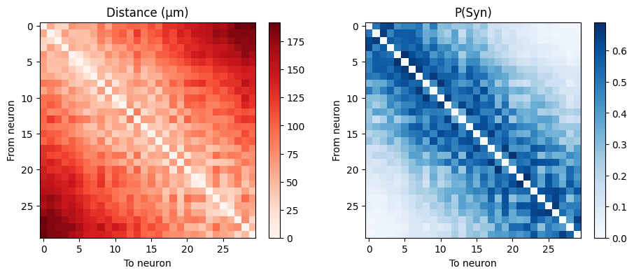
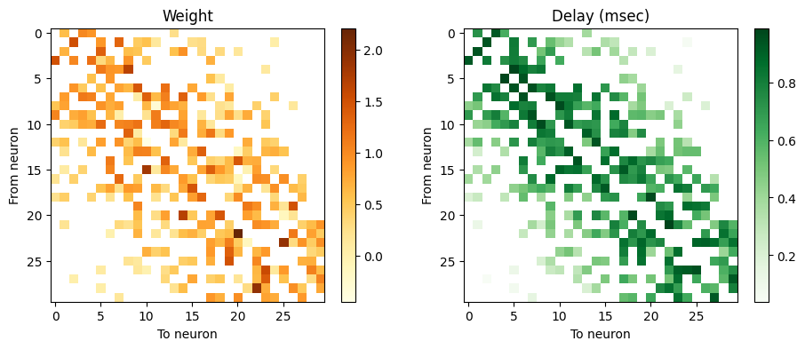
Let’s show the per-neuron-pair matrices of the factors involved.
First, tabulate the absolute distance, and the probability of a connection for each neuron pair:
%matplotlib inline
plt.close('all')
fig, axs = plt.subplots(nrows=1, ncols=2, figsize=(11,4));
axs[0].set_title('Distance (μm)'); im = axs[0].imshow(d_mat, cmap='Reds'); fig.colorbar(im, ax=axs[0]);
axs[1].set_title('P(Syn)'); im = axs[1].imshow(p_mat, cmap='Blues'); fig.colorbar(im, ax=axs[1]);
for i in range(axs.shape[0]): axs[i].set_ylabel('From neuron'); axs[i].set_xlabel('To neuron');
And now, tabulate weight and delay for the connections that were actually realized:
w_2d = np.zeros((N_cells,N_cells))*np.nan; d_2d = w_2d + 0 # full mask
w_2d[pre,post] = weight; d_2d[pre,post] = delay # fill in the values that apply

fig, axs = plt.subplots(nrows=1, ncols=2, figsize=(11,4));
axs[0].set_title('Weight'); im = axs[0].imshow(w_2d, cmap='YlOrBr'); fig.colorbar(im, ax=axs[0]); # could also use a diverging cmap centered at 0
axs[1].set_title('Delay (msec)'); im = axs[1].imshow(d_2d*1000, cmap='Greens'); fig.colorbar(im, ax=axs[1]);
for i in range(axs.shape[0]): axs[i].set_ylabel('From neuron'); axs[i].set_xlabel('To neuron');
Adding stimuli
Now let’s play with the network through unnatural means – for example, apply a one-off DC clamp to cells in the bottom 20% of the cylinder.
The attentive reader may have noticed that what’s been specified so far is not specific to NeuroML. That’s because NeuroML can run any distribution of cells and synapses just the same; they can be constructed independently with any method, and expressed in the NeuroML data format just before running the model.
The more involved and detailed descriptions(neuron shape, chemistry, dynamics and such) for the individual parts of the model will be specified in NeuroML, in the section right after.
stim_cells = [i for i, (x,y,z) in enumerate(cell_positions) if y < region_height/5]
stim_cells
[0, 1, 2, 3, 4, 5]
Generating NeuroML for the model
Now it’s time to make the NeuroML files in order to run the simulation. Let’s put them in a sub-folder of the working directory, to avoid polluting the folder that the notebook is in too much.
nml_dir = 'tut_net/'
os.makedirs(nml_dir, exist_ok=True)
For the cell’s description, let’s cheat and grab an existing description from the NeuroML-DB.
nmldb_cell_name = 'NMLCL000625'
zip_file_name = f'{nmldb_cell_name}.zip'
# Download the zip file with the model
import urllib.request
# Because NMLDB is having some issues with HTTPS, don't demand HTTPS verification
import ssl; ssl._create_default_https_context = ssl._create_unverified_context
urllib.request.urlretrieve(f'http://neuroml-db.org/GetModelZip?modelID={nmldb_cell_name}&version=NeuroML', zip_file_name)
# and unpack it
from zipfile import ZipFile
with ZipFile(zip_file_name, 'r') as zipp: zipp.extractall(nml_dir+nmldb_cell_name+'/')
NMLCLxxxxxx identifier. (Neither is the NML file)<name>.cell.nml filename, so let’s scan for that.<spikeThresh> to register an action potential is not specified for some reason. Because we’re using classical chemical synapses, we’ll have to add it to <biophysicalProperties>.
# LATER get it with libNML or with the NMLDB API.
import os
celltype_name = None
cell_nml_file_suffix = '.cell.nml'
for filename in os.listdir(nml_dir+nmldb_cell_name):
    # print(filename)
    if not filename.endswith(cell_nml_file_suffix): continue # get the cell.nml files
    new_celltype_name = filename[:-len(cell_nml_file_suffix)] # there it is
    if celltype_name: raise ValueError(f'cell type: is it {new_celltype_name} or {new_celltype_name}') # :c
    celltype_name = new_celltype_name
print('Celltype name:', celltype_name)

# Also modify the NML file to add spikeThresh
cell_filename = nml_dir+nmldb_cell_name+'/'+new_celltype_name+cell_nml_file_suffix
# Read in the file
with open(cell_filename, 'r') as file: filedata = file.read()
# Replace the target string
if '<spikeThresh' not in filedata:filedata = filedata.replace('</membraneProperties>','<spikeThresh value="0 mV"/></membraneProperties>')
# Write the file out again
with open(cell_filename, 'w') as file: file.write(filedata)
# print(filedata)
Celltype name: cACint209_L6_NBC_a3972c5d97_0_0
Now let’s add some routines to construct a NeuroML file incrementally from the population and projection data we collected so far, into one big string. There are also other ways to create and manipulate NeuroML files, but this one here makes for a more direct demonstration.
def NmlHeader():
    return '''<neuroml xmlns="http://www.neuroml.org/schema/neuroml2"  xmlns:xs="http://www.w3.org/2001/XMLSchema" xmlns:xsi="http://www.w3.org/2001/XMLSchema-instance" xsi:schemaLocation="http://www.neuroml.org/schema/neuroml2 https://raw.github.com/NeuroML/NeuroML2/development/Schemas/NeuroML2/NeuroML_v2.1.xsd">
    <include file="sim_components.nml"/>'''
def NmlNetworkHeader(): return '''\n   <network id="Net" type="networkWithTemperature" temperature="37degC">'''
def NmlNetworkFooter(): return '''\n    </network>'''

def NmlPopulation(pop_name, celltype_name, cell_positions):
    return f'''
        <population id="{pop_name}" component="{celltype_name}" size="{len(cell_positions)}">
        '''+'\n\t'.join([
            f'  <instance id="{i}"><location x="{x}" y="{y}" z="{z}"/></instance>'
            for i, (x,y,z) in enumerate(cell_positions) ])+'''
        </population>
    '''

def NmlSynapticProjection(
    proj_name,syncomp_name, pre_pop_name, post_pop_name,
    preCell, postCell, weight=None, delay=None, preSeg=None, postSeg = None, preFrac = None, postFrac = None):
    if delay is None: delay = [0]*len(preCell)
    if weight is None: weight = [1]*len(preCell)
    if preSeg is None: preSeg = [0]*len(preCell)
    if postSeg is None: postSeg = [0]*len(preCell)
    if preFrac is None: preFrac = [0]*len(preCell)
    if postFrac is None: postFrac = [0]*len(preCell)

    return f'''
        <projection id="{proj_name}" synapse="{syncomp_name}" presynapticPopulation="{pre_pop_name}" postsynapticPopulation="{post_pop_name}">
            '''+'\n\t    '.join([
            f'<connectionWD id="{i}" preCellId="{preCell[i]}" postCellId="{postCell[i]}" '+
            f'weight="{weight[i]}" delay="{delay[i]} s" '+
            f'preSegmentId="{preSeg[i]}" postSegmentId="{postSeg[i]}" '+
            f'preFractionAlong="{preFrac[i]}" postFractionAlong="{postFrac[i]}"/>'
            for i in range(len(pre)) ])+'''
        </projection>
    '''

def NmlInputList(input_list_name,stim_component,target_pop_name,cells, segs=None, fracs=None):
    if segs is None: segs = [0]*len(cells)
    if fracs is None: fracs = [0]*len(cells)
    return f'''
        <inputList id="{input_list_name}" population="{target_pop_name}" component="{stim_component}">
        '''+'\n\t'.join([
            f'  <input id="{i}" target="../{target_pop_name}[{cells[i]}]" '+
            f'segmentId="{segs[i]}" fractionAlong="{fracs[i]}" destination="synapses"/>'
            for i in range(len(cells)) ])+'''
        </inputList>
    '''

def NmlFooter():return '''\n</neuroml>'''

# celltype_name = 'cACint209_L6_NBC_a3972c5d97_0_0'
# celltype_name = 'cADpyr232_L5_TTPC2_8bab918b58_0_0'
# celltype_name = 'dNAC222_L6_SBC_194972ee43_0_0'

population_name = 'MyCells'

# Write the network file.
with open(nml_dir+"/example.nml", "w") as f:
    f.write(NmlHeader()); f.write(NmlNetworkHeader())
    f.write(NmlPopulation(population_name, celltype_name, cell_positions))
    f.write(NmlSynapticProjection('FirstSynProjection', 'NMDA', population_name, population_name, pre, post, weight, delay))
    f.write(NmlInputList('FirstStimList', 'MyStim', population_name, stim_cells))
    f.write(NmlNetworkFooter())
    f.write(NmlFooter())
After writing the net.nml representing the network made up of cells, synapses and input stimuli, we’ll make a companion file LEMS_<something>.xml (this is the convention; I guess you could also use .sim.xml to make the name further clearer.)
Here, we’ll specify some parameters to run the simulation like for how long and with how big a timestep, but also add the last part of the rig: recording certain trajectories and spike trains from the simulated model. Since neurites in each cell usually fire together(in sequence), we’ll record the membrane voltage trajectories for the soma of each neuron. (Conveniently enough, if the location on the neuron is not specified in a NeuroML path, the location of the soma is used.)
# Write the sim file.
def NmlSimParms(pop_name, N_cells, run_time, run_timestep=25e-6):
    return f'''
        <Simulation id="sim1" length="{run_time}s" step="{run_timestep}s" target="Net">
            <OutputFile id="first" fileName="tut_net/results.gen.txt">
            '''+'\n\t        '.join([f'<OutputColumn id="v_{i}" quantity="{pop_name}[{i}]/v"/>' for i in range(N_cells)])+'''
            </OutputFile>
        </Simulation>
        <Target component="sim1"/>'''

with open(nml_dir+"/Sim.xml", "w") as f:
    f.write('<?xml version="1.0" encoding="UTF-8"?>\n<Lems>\n<include file="example.nml"/>\n')
    f.write(NmlSimParms(population_name, N_cells, run_time=0.25, run_timestep=25e-6))
#     f.write(NmlSimParmss(population_name,celltype_name,None, run_time=0.25, run_timestep=25e-6))
    f.write('\n</Lems>\n')
%%writefile $nml_dir/sim_components.nml
<neuroml>
    <include file="NMLCL000625/cACint209_L6_NBC_a3972c5d97_0_0.cell.nml"/>
    <expTwoSynapse id="NMDA" gbase=".5nS" erev="0mV" tauDecay="15ms" tauRise="0.15ms"/>
    <pulseGenerator id="MyStim" delay="10ms" duration="20ms" amplitude="0.5nA"/>
</neuroml>
Writing tut_net//sim_components.nml
Here are some more tested parameter combinations for alternative cell types. You can replace the nmldb_cell_name above, download a new neuron model, then uncomment and run the corresponding snippet in place of the code above. Or even get a new cell type from other sources, such as NeuroML-DB, OSB or the internet in general.
# %%writefile nml_sim/sim_components.nml
# <neuroml>
#     <include file="NMLCL000693/cADpyr232_L5_TTPC2_8bab918b58_0_0.cell.nml"/>
#     <expTwoSynapse id="NMDA" gbase="6.5nS" erev="0mV" tauDecay="15ms" tauRise="0.15ms"/>
#     <pulseGenerator id="MyStim" delay="10ms" duration="50ms" amplitude="1.5nA"/>
# </neuroml>
# %%writefile nml_sim/sim_components.nml
# <neuroml>
#     <include file="NMLCL001078/dNAC222_L6_SBC_194972ee43_0_0.cell.nml"/>
#     <expTwoSynapse id="NMDA" gbase="0.57nS" erev="-0mV" tauDecay="17ms" tauRise="0.05ms"/>
#     <pulseGenerator id="MyStim" delay="10ms" duration="100ms" amplitude="0.2nA"/>
# </neuroml>
import eden_simulator
%time results = eden_simulator.runEden(nml_dir+"/Sim.xml")
CPU times: user 108 ms, sys: 9.11 ms, total: 117 ms
Wall time: 11.8 s
Let’s see what we got out of the simulation:
print(results.keys())
dict_keys(['MyCells[0]/v', 'MyCells[1]/v', 'MyCells[2]/v', 'MyCells[3]/v', 'MyCells[4]/v', 'MyCells[5]/v', 'MyCells[6]/v', 'MyCells[7]/v', 'MyCells[8]/v', 'MyCells[9]/v', 'MyCells[10]/v', 'MyCells[11]/v', 'MyCells[12]/v', 'MyCells[13]/v', 'MyCells[14]/v', 'MyCells[15]/v', 'MyCells[16]/v', 'MyCells[17]/v', 'MyCells[18]/v', 'MyCells[19]/v', 'MyCells[20]/v', 'MyCells[21]/v', 'MyCells[22]/v', 'MyCells[23]/v', 'MyCells[24]/v', 'MyCells[25]/v', 'MyCells[26]/v', 'MyCells[27]/v', 'MyCells[28]/v', 'MyCells[29]/v', 't'])
Displaying per-soma activity
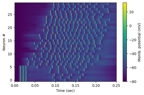
Let’s show how each cell behaved during the simulation, with an analog raster.
We observe that the bottom few cells were stimulated together, fired together and then entered a refractory period; meanwhile the other cells stimulate one another into a wave that spreads out (in spatial order!), reverberates for some time, and dies out near the end of the simulation.
Observe also the sub-threshold behavior; the cells were gradually brought to a depolarisation level before they started firing repetitively.
neuron_waveforms = np.array([results[f'{population_name}[{i}]/v'] for i in range(N_cells)])
neuron_appearance_order = np.argsort(cell_positions[:,1]) # just in case they weren't sorted before
# neuron_appearance_order = range(N_cells) # alternative order, if not sorted
fig = plt.figure(figsize=np.array([8,5])*.8); ax = plt.gca()
im = plt.imshow(1000*neuron_waveforms[neuron_appearance_order,:], # in mVolts
    extent=[ results['t'][0], results['t'][-1], N_cells-.5,-0.5 ],
    aspect='auto', interpolation='none', cmap ="viridis")
cbar = plt.colorbar(im); cbar.set_label('Memb. potential (mV)')
ax.set_xlabel('Time (sec)'); ax.set_ylabel('Neuron #')
ax.invert_yaxis() # to match the cell positions' 'up' in 3-D space
plt.show(); fig.savefig('tut_net_raster.png',dpi=300)
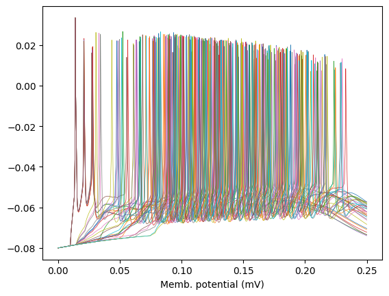
Here’s an alternative line plot, to see how it gets unwieldy for large population sizes: (it could be ameliorated with a EEG style vertical offset, at the cost of resolution though)
fig = plt.figure()
plt.plot(results['t'], neuron_waveforms.T, linewidth=.5)
plt.xlabel('Time (s)');plt.xlabel('Memb. potential (mV)');plt.show()
fig.savefig('tut_net_jumble.png',dpi=300)
Since we have the cells’ positions, we can display soma potential in 3-(4 including time)-D space as well.
First, we should reduce the amount of data to display to what’s perceiveable at the animation speed we choose, i.e. downsample the recorded waveforms in time. Note that this was already done previously, through the plt.figure’s parameters for figsize and dpi. This is neatly done by the auxiliary 𝚎𝚍𝚎𝚗_𝚜𝚒𝚖𝚞𝚕𝚊𝚝𝚘𝚛.𝚍𝚒𝚜𝚙𝚕𝚊𝚢.𝚊𝚗𝚒𝚖𝚊𝚝𝚒𝚘𝚗.𝚜𝚞𝚋𝚜𝚊𝚖𝚙𝚕𝚎_𝚝𝚛𝚊𝚓𝚎𝚌𝚝𝚘𝚛𝚒𝚎𝚜 routine, that comes with the
𝚍𝚒𝚜𝚙𝚕𝚊𝚢 section of the Python API.
from eden_simulator.display.animation import subsample_trajectories
samples, anim_axis, sampled_time_axis, [sampled_soma_voltage] = subsample_trajectories(
    results['t'], [neuron_waveforms.T * 1000], animation_speed=0.03, animation_frames_per_second=60)
Then we’ll display the waveforms as an animated 3D scatter plot, using 𝚔𝟹𝚍.𝚙𝚘𝚒𝚗𝚝𝚜. We’ll also use 𝚎𝚍𝚎𝚗_𝚜𝚒𝚖𝚞𝚕𝚊𝚝𝚘𝚛.𝚍𝚒𝚜𝚙𝚕𝚊𝚢.𝚜𝚙𝚊𝚝𝚒𝚊𝚕.𝚔𝟹𝚍.𝙿𝚕𝚘𝚝 and 𝙸𝙿𝚢𝚝𝚑𝚘𝚗.𝚍𝚒𝚜𝚙𝚕𝚊𝚢.𝙷𝚃𝙼𝙻 for improved publishing.
import k3d; from eden_simulator.display.spatial.k3d import Plot
Point_plot = plot = Plot(camera_auto_fit=False) # to override camera orientation

k3d_anim_dict = { str(real_time): x.astype(np.float32)
                for (real_time, x) in zip(anim_axis, sampled_soma_voltage)  }
k3d_label_dict = { str(real): f't = {sim:.3f} ~ s' for (real, sim) in zip(anim_axis, sampled_time_axis)  }
plt_points = k3d.points(positions=cell_positions.astype(np.float32),attribute=k3d_anim_dict,
        color_range=[-80, +20],point_size=10,color_map=k3d.matplotlib_color_maps.Rainbow); plot += plt_points

plot.camera = plot.get_auto_camera(pitch=30, yaw=10)[:6]+[0,1,0] # set 'y' to up !  LATER zoom a bit also; vecs are pos, tgt, up
plt_label = k3d.text2d(k3d_label_dict, (0.,0.), label_box=False); plot += plt_label # add 2d elements AFTER setting auto camera
plot.fps = 60;
from IPython.display import display, HTML, IFrame
plot.snapshot_type = 'inline'; display(HTML(plot.get_snapshot()))
But this doesn’t look much like the tissue we’re supposed to simulate, does it? We have spent all this computer time to simulate all these neurites making up the cell, we deserve more attractive visuals!
Let’s move on then to display the membrane voltage all over the cell, in glorious, 24 bit, false color! (You’d need fluo to see it on the real thing anyway.)
Displaying whole-neuron activity
explain how spatially detailed cells are being simulated as discrete elements of neurite,
and how exactly these parts and the whole neuron look like as polygonal solids.
See also the chapter which explains the structure of spatially-detailed neurons, and introduces and uses said tools.
First, we’ll retrieve for this cell type, how many compartments is is cut into. Each compartment in a model neuron is equivalent to a pixel in an image; it is a (hopefully) small bit of the neuron where we assume all electrical, chemical etc. properties are uniform throughout.
We can get this as follows:
cells_info = eden_simulator.experimental.explain_cell(nml_dir+"/Sim.xml")
print(type(cells_info))
print(cells_info.keys())
cell_info = cells_info[celltype_name]
print(cell_info.keys())
<class 'dict'>
dict_keys(['cACint209_L6_NBC_a3972c5d97_0_0'])
dict_keys(['comp_parent', 'comp_start_pos', 'comp_end_pos', 'comp_midpoint', 'comp_midpoint_segment', 'comp_midpoint_fractionAlong', 'comp_length', 'comp_path_length_from_root', 'comp_area', 'comp_volume', 'comp_capacitance', 'comp_conductance_to_parent', 'segment_groups', 'mesh_vertices', 'mesh_faces', 'mesh_comp_per_face'])
For each physically modelled* cell type, we got a set of lists, most with as many elements as there are compartments for each cell type. We can then use the comp_midpoint_segment and comp_midpoint_fractionAlong lists to locate the middle of each compartment, and tap into that to record the membrane voltage for each part of each neuron.
Given this information, let’s record for each cell. We’ll also cut down on the sampling rate (using the Eden-specific extension <EdenOutputFile>) because that’s way more than the one trajectory per cell we were recording before.
To learn more about explain_cell, refer to its Python API page.
* that is, excluding artificial cells which typically have unique properties
comp_mid_seg = cell_info['comp_midpoint_segment']
comp_mid_fra = cell_info['comp_midpoint_fractionAlong']
n_comps = len(comp_mid_seg) # Number of actual compartments in this cell, may be retrieved from most cell_info arrays
print(f'{n_comps} compartments per cell')
202 compartments per cell
Now we’ll construct a SimMore.xml file that records the voltage of every single compartment on every single cell.
We’ll also cut down how often we record these waveforms to 0.5 msec (default NeuroML behaviour is to record for every single timestep which is quite a lot of steps, and we don’t always need this much resolution.)
Note the use of <EdenOutputFile>, an EDEN-specific version of the regular <OutputFile> with more recording options. Another one of these is controlling the units per recorded trajectory in output_units, which we’ll use to record membrane voltage in the more commonly used millivolts, this time.
# Set a new routine for making the <Simulation> file with new recording options
def NmlSimParmss(run_time, run_timestep=25e-6, sampling_period=1e-3,
            rec_lines='', href='file://results.gen.txt'):
    return f'''
        <Simulation id="sim1" length="{run_time}s" step="{run_timestep}s" target="Net">
            <EdenOutputFile id="first" href="{href}" format="ascii_v0" sampling_interval="{sampling_period} s">
            '''+'\n\t        '.join(rec_lines)+'''
            </EdenOutputFile>
        </Simulation>
        <Target component="sim1"/>'''

# Make the traces to record each compartment, and save the file
traces = [f"{population_name}[{neu}]/{celltype_name}/{comp_mid_seg[i]}{('%.9f'%comp_mid_fra[i])[1:]}/v"
    for neu in range(N_cells) for i in range(len(comp_mid_seg))]
rec_lines = [f'<OutputColumn id="v_{i}" quantity="{x}"  output_units="mV"/>' for i,x in enumerate(traces) ]
print(f"recording {len(rec_lines)} waveforms this time !")
with open(nml_dir+"/SimMore.xml", "w") as f:
    f.write('<?xml version="1.0" encoding="UTF-8"?>\n<Lems>\n<include file="example.nml"/>\n')
    f.write(NmlSimParmss(run_time=0.25, run_timestep=25e-6, sampling_period=0.5e-3, href='./moresults.gen.txt', rec_lines=rec_lines))
    f.write('\n</Lems>\n')
recording 6060 waveforms this time !
%time moresults = eden_simulator.runEden(nml_dir+"/SimMore.xml",verbose=True)
Using bundled executable: on /home/docs/checkouts/readthedocs.org/user_builds/eden-simulator/envs/latest/lib/python3.10/site-packages/eden_simulator/data/bin/eden
['/home/docs/checkouts/readthedocs.org/user_builds/eden-simulator/envs/latest/lib/python3.10/site-packages/eden_simulator/data/bin/eden', 'nml', 'tut_net//SimMore.xml', 'gcc']
Ran EDEN in 12.48 seconds
CPU times: user 318 ms, sys: 64.2 ms, total: 383 ms
Wall time: 12.9 s
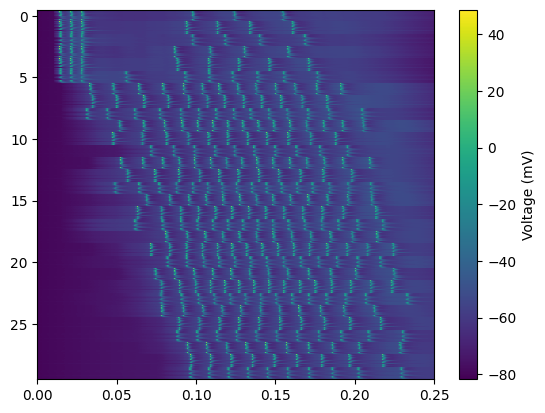
Now we have many more traces in the sim output, one per neuron per compartment!
Just in case we want differently-shaped neurons in the future, let’s leave the traces list to be:
instead of making an array of
N_cells x n_comps x timesteps, assign an index number in the sequence of traces, from which the set of traces start (n_comps trajectories, including the indexed one)
from matplotlib import pyplot as plt
neuron_waveforms = np.array([moresults[x] for i,x in enumerate(traces)])
print('Waveform matrix size:', neuron_waveforms.shape)
# XXX append the offsets
timevec = moresults['t']
offset_per_neuron = np.round(np.arange(N_cells)*n_comps)
print('Row start per cell:', offset_per_neuron)
im = plt.imshow(neuron_waveforms,
    extent=[ results['t'][0], timevec[-1], N_cells-.5,-0.5 ],
    aspect='auto', interpolation='none', cmap ="viridis");cbar = plt.colorbar(im); cbar.set_label('Voltage (mV)')
Waveform matrix size: (6060, 501)
Row start per cell: [   0  202  404  606  808 1010 1212 1414 1616 1818 2020 2222 2424 2626
 2828 3030 3232 3434 3636 3838 4040 4242 4444 4646 4848 5050 5252 5454
 5656 5858]
When we ran explain_cell, some lists mesh_vertices, mesh_faces and mesh_comp_per_face were also provided for the cell. These represent the solid shape (in computer graphics parlance, a mesh) that cells of this type have. (For unique morphology, one would make individual cell types in NeuroML.)
Meshes are made up from a set of points (known as vertices) in 3-D space, and a set of polygonal faces (typically triangles). Thus the joined flat faces form the shape together, just like lines connected through lines do in 2D space. To display a 3-D object, meshes may be enhanced with texture images and related attributes, to show a more detailed surface on the meshes. But for our purpose, we’ll be painting the mesh explicitly, so that we can show biophysical attributes across each cell.
mesh_vertices = cell_info['mesh_vertices']
mesh_faces    = cell_info['mesh_faces'   ]
import trimesh
viz = trimesh.Trimesh(
    vertices=mesh_vertices, faces=mesh_faces )
viz.visual.face_colors = (0.1,0.9,0.1)
viz.show()
Note that that if \(z\) is up, that’s a different orientation compared to the render in the NeuroML-DB.
For the following, we’ll assume \(\,\overrightarrow y~\) points to “up” and rotate the plot.camera accordingly, just like we did in the previous point-based animation. (For more about the meaning of each coordinate axis, refer to the article on spatially-detailed cells.)
In addition to the mesh’s vertices and faces we got a list mesh_comp_per_face, which indicates which compartment is represented by each face of the mesh.
face_comp = cell_info['mesh_comp_per_face']
print(f"We have {len(mesh_faces)} faces in the mesh, and {len(face_comp)} matching labels.")
We have 30148 faces in the mesh, and 30148 matching labels.
Combining this with the vertex numbers that each face is made of, we can have both a mapping from each compartment to each corresponding face, as well as from each compartment to each vertex. (Different 3D graphics utilities prefer each form.)
We’ll now use this mapping to paint the neuron selectively, with a different colour for each compartment, to show how membrane potential spreads when it’s initiated from the soma. This can be done immediately through the auxiliary 𝚎𝚍𝚎𝚗_𝚜𝚒𝚖𝚞𝚕𝚊𝚝𝚘𝚛.𝚍𝚒𝚜𝚙𝚕𝚊𝚢.𝚜𝚙𝚊𝚝𝚒𝚊𝚕.𝚔𝟹𝚍.𝚙𝚕𝚘𝚝_𝚗𝚎𝚞𝚛𝚘𝚗 routine, that comes with the 𝚍𝚒𝚜𝚙𝚕𝚊𝚢 section of the Python API.
Tip: When animating a spatially neuron over many time samples, use compress_cells = True(default) with plot_neuron and display it on a eden_simulator.display.spatial.k3d.Plot with IPython.display.HTML or IPython.display.IFrame to keep the memory and space requirements under control.
from eden_simulator.display.animation import subsample_trajectories
_, anim_axis, sampled_time_axis_sec, (sampled_voltage,) = subsample_trajectories(
    timevec, [neuron_waveforms.T], animation_speed=0.03, animation_frames_per_second=60)

import k3d; from eden_simulator.display.spatial.k3d import Plot, plot_neuron
Multicomp_plot = plot = Plot()
k3d_label_dict = { str(real): f't = {sim:.3f} ~ s' for (real, sim) in zip(anim_axis, sampled_time_axis_sec)  }
for neu in range(N_cells):
    tra_off = offset_per_neuron[neu] # some traces per neuron, starting from ...
    comp_trajes = sampled_voltage[:,tra_off:tra_off+n_comps] # there they are
    plot += plot_neuron(cell_info, comp_trajes, time_axis_sec=anim_axis, translation=cell_positions[neu,:],
                            color_range=[-80, 0],color_map='rainbow');
plot.camera = plot.get_auto_camera(pitch=30, yaw=10)[:6]+[0,1,0] # set 'y' to up !  LATER zoom a bit also; vecs are pos, tgt, up
plt_label = k3d.text2d(k3d_label_dict, (0.,0.)); plot += plt_label # add 2d elements AFTER setting auto camera

# Since the plot is quite big, include it outside of the notebook so that the notebook renders quick.
plot.snapshot_type = 'online'; plot_html = plot.get_snapshot()
plot_file = '_static/tutorial_network_big_animation.html'
with open(plot_file, 'w') as f: f.write(plot_html)
display(IFrame('_static/tutorial_network_big_animation.html', '100%', f'{plot.height} px'))
Observe how the spikes travel along the neurites.
Exercise: While constructing the model (before implementing the NeuroML description), there was a mistake in one of the formulae for the network parameters. This mistake makes whether the neurons’ spatially reverberating waves occur, extremely sensitive to the physical parameters of the neuron model, synapses and applied probes.
Find the mistake and re-evaluate sensitivity (also with the alternative cell types commented out above) using the corrected, plausible formula. If a fine-tuned, wrong model can reproduce the expected phenomenon, what does that imply for computational neuroscience?