.
.
 Download notebook.
Tutorial: A balanced excitatory-inhibitory network with delta synapses
A popular network dynamics model involves two interconnected populations of neurons: those in the first “excitatory” population stimulate (depolarise) all post-synaptic neurons, while neurons of the “inhibitory” population suppress (repolarise) all their post synaptic neurons, whether they are excitatory or inhibitory. Various interesting patterns can emerge out of such systems, depending on the particular parameters of the excitation-inhibition balance. A macro-scale, rate-based formulation is the Wilson-Cowan model. A more detailed formulation with LIF point neurons, impulse-based synapses, and stochastic external input has been studied by Brunel: on paper regarding general statistics and equilibria, but also with numerical simulations for interesting parameter combinations.
This chapter shows how to model such a network using EDEN. The network can be expressed in conventional NeuroML – save for the post-synaptic effect, which is modelled as instantaneous jumps in membrane potential or impulses of current. This effect could be approximated with short enough current pulses (as the numerical schemes used allow); but now it can also be declared precisely, thanks to EDEN’s <WritableRequirement> extension to NeuroML.
Note that the same synapse model can be used for both inter-neuron synaptic <projection>s, as well as for the excitatory <poissonFiringSynapse>s driving the cell; the semantics are preserved.
First, let’s set up the network’s parameters. We’ll opt for asynchronous firing for this example:
# Adapted from the Brian adaptation: https://brian2.readthedocs.io/en/stable/examples/frompapers.Brunel_2000.html
sim_duration = 0.1 # just for demonstration
# network parameters
N_exc = 4000 # NB: the original paper shows for 10000, the behaviour doesn't change that much
N_inh = int(N_exc/4)
p_connections = 0.1
N_ext_inputs = int(round(p_connections * N_exc))

# Cell parameters in SI units
cell_tau = 20e-3 # sec
cell_vth = 20e-3 # volt
cell_vr  = 10e-3 # volt
cell_ref =  2e-3 # sec

# synapse parameters
syn_delta = 0.1e-3 # volt
conn_delay = 1.5e-3 # sec

# system state parameters
# for asynchronous spiking
g = 5 # relative inhibitory to excitatory synaptic strength
nu_ext_over_nu_thr = 2 # ratio of external stimulus rate to threshold rate

# derived properties
nu_thr = cell_vth / (syn_delta * N_ext_inputs * cell_tau) # hertz
# external stimulus
nu_ext = nu_ext_over_nu_thr * nu_thr
# N_ext_inputs at a rate of nu_ext and weight of syn_delta for every cell
Then let’s define the cell and synapse models:
cell_defs = f'''
<ComponentType name="VoltTauCell" extends="baseCellMembPotCap"> <!-- not really cap but since baseSynapse exposes current... -->
    <Parameter name="v_reset" dimension="voltage"/>
    <Parameter name="v_thresh" dimension="voltage"/>
    <Parameter name="tau_mem" dimension="time"/>
    <Parameter name="tau_refrac" dimension="time"/>
    <Dynamics>
            <StateVariable name="lastSpikeTime" dimension="time"/>
        <StateVariable name="v" dimension="voltage" exposure="v"/>

        <ConditionalDerivedVariable name="voltage_rate" dimension="voltage_per_time">
                    <Case condition="t .gt. lastSpikeTime + tau_refrac" value="(-v) / tau_mem"/>
                    <Case value="0"/>
            </ConditionalDerivedVariable>
            <TimeDerivative variable="v" value="voltage_rate" />

        <OnStart> <!-- Start at resting state -->
            <StateAssignment variable="v" value="v_reset"/> <!-- TODO or zero? -->
            <StateAssignment variable="lastSpikeTime" value="t - tau_refrac" />
        </OnStart>

            <OnCondition test="(v .gt. v_thresh) .and. (t .gt. lastSpikeTime + tau_refrac)">
                    <EventOut port="spike"/>
                    <StateAssignment variable="lastSpikeTime" value="t" />
                    <StateAssignment variable="v" value="v_reset" />
            </OnCondition>
    </Dynamics>
</ComponentType>
<VoltTauCell id="IafTauRefNeuron" tau_mem="{cell_tau} s" tau_refrac="{cell_ref} s" v_thresh="{cell_vth} V" v_reset="{cell_vr} V"  C="0.2nF" /> <!-- C is unused, see above -->
'''
syns_defs = f'''
<ComponentType name="DeltaSyn" extends="baseSynapse" description="A voltage-impulse synapse model. In case cell capacitance is variable, consider a current-impulse model instead.">
    <Constant name="AMP" dimension="current" value="1 A"/>
    <Parameter name="delta" dimension="voltage" description="Weight really"/> <!-- TODO access the weight of the synapse as defined on the projection, somehow! -->
    <WritableRequirement name="v" dimension="voltage"/>
    <Dynamics>
            <DerivedVariable name="i" exposure="i" dimension="current" value="0 * AMP" />
            <OnEvent port="in">
                    <StateAssignment variable="v" value="v+delta"/>
            </OnEvent>
    </Dynamics>
</ComponentType> <!-- TODO updating., init weight, etc. -->
<DeltaSyn id="SynExc" delta="{syn_delta} V"/>
<DeltaSyn id="SynInh" delta="{-g*syn_delta} V"/>
'''
Then generate the synaptic projections between populations. (Note that the XML format starts to become a nuisance for several million synapses…)
import numpy as np
rng = np.random.default_rng(seed=5)
def RandomUniformProjection(rng, N_from, N_to, prob, symmetric):
    M = rng.uniform(size=(N_from,N_to))
    if symmetric: M += np.eye(N_from, N_to) # exclude diagonal
    ei, ej = np.where(M < prob)
    return ei, ej

popsizes = {'Exc': N_exc, 'Inh': N_inh}
def get_synapses(projname, source, target, syntype, weight=1, delay_sec=0, prob=0.1):
    nml_lines = [f'''\t<projection id="{projname}" presynapticPopulation="{source}" postsynapticPopulation="{target}" synapse="{syntype}">''']
    syn_i, syn_j = RandomUniformProjection(rng, popsizes[source], popsizes[target], prob, (source == target))

    nml_lines +=  [ f'\t\t<connectionWD id="{ii}" preCellId="{pre}" postCellId="{post}" weight="{weight}" delay="{delay_sec} s"/>' for ii, (pre, post) in enumerate(zip(syn_i, syn_j))]
    nml_lines += ['\t\t</projection>']
    return nml_lines, len(syn_i)
net_lines = []
net_ee, n_ee = get_synapses("ee_synapses", 'Exc', 'Exc', 'SynExc', weight=+1, delay_sec=conn_delay, prob=p_connections); net_lines += net_ee
net_ei, n_ei = get_synapses("ei_synapses", 'Exc', 'Inh', 'SynExc', weight=+1, delay_sec=conn_delay, prob=p_connections); net_lines += net_ei
net_ie, n_ie = get_synapses("ie_synapses", 'Inh', 'Exc', 'SynInh', weight=-g, delay_sec=conn_delay, prob=p_connections); net_lines += net_ie
net_ii, n_ii = get_synapses("ii_synapses", 'Inh', 'Inh', 'SynInh', weight=-g, delay_sec=conn_delay, prob=p_connections); net_lines += net_ii
Then assemble the NeuroML components, the synaptic projections, and many many (N_ext_inputs) independently firing external synapses attached to each neuron, into the model file:
tabline = '\n    ' # annoyingly enough, \ may not exist at all in a f string, not even in brackets. Fixed in Python 3.12+
nml_file=''
nml_file=f'''
<neuroml>

{cell_defs}
{syns_defs}
<poissonFiringSynapse id="PoissonInput" averageRate="{nu_ext} Hz" synapse="SynExc" spikeTarget="./GenericDeltaSynExc"/>

<network id="Net">
    <population id="Exc" component="IafTauRefNeuron" size="{N_exc}"/>
    <population id="Inh" component="IafTauRefNeuron" size="{N_inh}"/>

    {tabline.join(net_lines)}

    <inputList id="InpExc" population="Exc" component="PoissonInput">
        {tabline.join([ f'<input id="{i}" target="Exc[{idx}]" destination="synapses"/>' for i, idx in enumerate([cell for cell in range(N_exc) for jjj in range(N_ext_inputs)]) ])}
    </inputList>
    <inputList id="InpInh" population="Inh" component="PoissonInput">
        {tabline.join([ f'<inputW id="{i}" target="Inh[{idx}]" destination="synapses" weight="1"/>' for i, idx in enumerate([cell for cell in range(N_inh) for jjj in range(N_ext_inputs)]) ])}
    </inputList>
</network>
</neuroml>
'''
with open('Model.nml', 'wt') as f: f.write(nml_file)

sim_file = f'''<Lems><include href="Model.nml"/><Simulation id="MySim" length="{sim_duration} s" step="100 us" target="Net">
    <EventOutputFile id="SpikesExc" fileName="spikes_exc.gen.txt" format="TIME_ID">
        {tabline.join([ f'<EventSelection id="{i}"  select="Exc[{i}]" eventPort="spike"/>' for i in range(N_exc)])}
    </EventOutputFile>
    <EventOutputFile id="SpikesInh" fileName="spikes_inh.gen.txt" format="TIME_ID">
        {tabline.join([ f'<EventSelection id="{i}"  select="Inh[{i}]" eventPort="spike"/>' for i in range(N_inh)])}
    </EventOutputFile>
</Simulation>
<Target component="MySim"/></Lems>'''
with open('Sim.nml', 'wt') as f: f.write(sim_file)

# it's quite big until we use h5 so let's save space
del nml_file, net_lines, net_ee, net_ii, net_ei, net_ie
import gc; gc.collect();
And run the simulation:
import eden_simulator as eden
tra, eve = eden.runEden('Sim.nml', reload_events=True, threads=1)
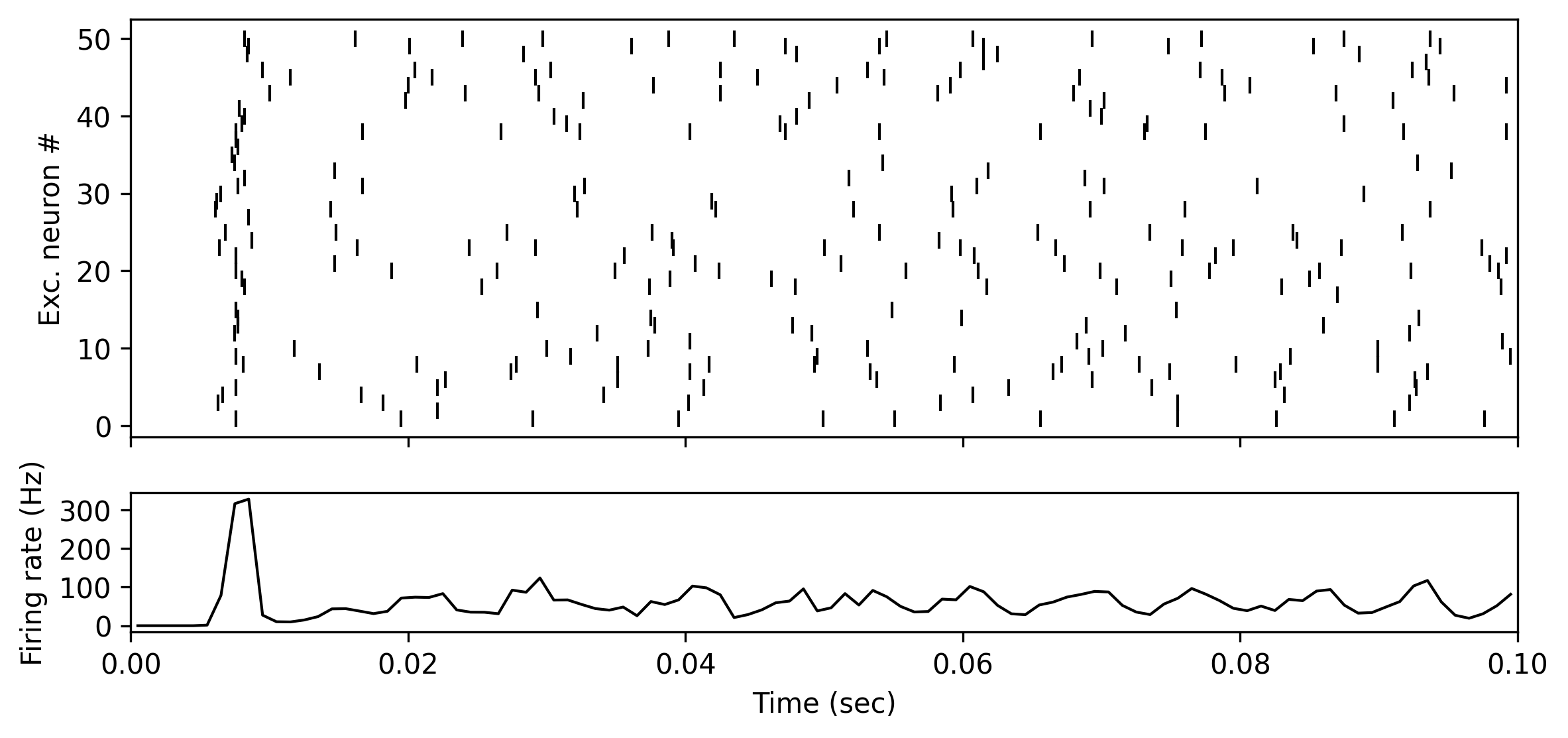
Let’s see the raster plot of the first 50 excitatory neurons. Since connectivity is the same over the whole population, they should represent a random sample. And also the firing rate of the whole population, using a histogram. (Could also use sliding window or other convolutions but it’s also good with enough bins)
import matplotlib; from matplotlib import pyplot as plt
fig, axs = plt.subplots(2,1,sharex=True,figsize=[9,4],height_ratios=[3,1], dpi=300)
for i in range(50):
    spikes=eve[f'Exc[{i}]']
    axs[0].plot(spikes, [i+1]*len(spikes), "|k")
axs[0].set_xlim([0,sim_duration]); axs[0].set_ylabel('Exc. neuron #');
binsize = 0.001 # seconds
counts, _ = np.histogram(
    [t for i in range(N_exc) for t in eve[f'Exc[{i}]']],
    range=[0,sim_duration], bins = round(sim_duration/binsize))
axs[1].plot((np.arange(len(counts))+.5)*binsize, counts/(N_exc*binsize),'-k',lw=1)
# axs[1].locator_params(axis='y', nbins=6)# axs[1].set_ylim([0, 130]);
axs[1].set_xlim(0, sim_duration)
axs[1].set_ylabel('Firing rate (Hz)'); axs[1].set_xlabel('Time (sec)');
axs[1].yaxis.set_major_locator(matplotlib.ticker.MultipleLocator(base=100))
# axs[1].axhline((1+nu_ext_over_nu_thr)*nu_thr,ls='--',c='orange')