Example: Reward-modulated STDP in a virtual environment - Brzosko, Zannone et al. (2017)
The brain is said to have smart neural structures which somehow learn, or at least adapt, to their surroundings and lead to – however basic – intelligent behaviours.
Can we see this in action? The neural network in Brzosko, Zannone et al. (2017) (code) learns to navigate toward a target, and then unlearn and relearn to reach a different target, with only whether the target has been reached as feedback.
This model learns to navigate with sequential reward-modulated STDP. Time is segmented into trials of the navigation task, and synapses are reinforced according to a time-symmetric “fire together, wire together” rule – but only at the end of each trial, and only if they succeeded. Meanwhile, spikes in general depress the involved synapses regardless of timing: this is how the SNN can unlearn unproductive behaviours, which will prove handy once the target location changes without warning after several trials. Finally, weights are constrained between a maximum and minimum positive value.
Navigation happens in a (simulated, for now) physical environment. Its dynamics are so simple that it could be implemented in LEMS, but here we’ll demonstrate how a SNN simulation can be plugged into any arbitrary environment: think of OpenAI Gym, the Metaverse or even real life.
In the following, we’ll get to (show how to) employ the following extensions to NeuroML:
Per-cell variability: so that place cells are selective to different locations;
<VariableReference>: to plug the agent’s location into the place cells’ activity;
Streaming I/O: to interact with another external process, which runs the mechanical simulation in tandem;
Accessing a point neuron’s state variables from a synapse: for both delta synapses and as a workaround, so that post-synapses can observe non-standard state variables of their neuron.
Architecture of the model and experimental rig
The model is basically an embodied A.I. agent, in terms of buzzwords: its physical presence or body is modelled as a freely-moving point in 2-dimensional space, which is guided by a spiking neural network (SNN) which is the “brains” for the body.
The SNN has two layers of neurons: The input layer has “place cells” which fire selectively to the body’s location, and the output layer has “action cells” which each select a direction of travel for the body. All input cells project to all action cells, with synaptic weights adjusted during simulation. Action cells project to other cells; their influence is mutually inhibitory for dissimilar directions, and excitatory for similar ones.
The body follows the direction pointed to by the SNN’s action cells (weighted by firing rate), while being physically limited to its rectangular-shaped playing field. Synapses from place cells associated with walls, to directions toward said walls, are excluded from the SNN, to prevent our agent from getting stuck. (Here’s an assignment for later, relax this crutch.)
Our experimental setup looks like this:

Implementing the model
To begin with, the synapses connecting the input layer to the output layer inject bi-exponentially-decaying current - but there is a quirk in the original code: when an output neuron fires, all inbound synapses are silenced instantly! We could have the synapse models peek into the cells to detect such spikes (as we’ll have to later on for STDP). But we’ll take this chance to show how exponential-current synapse models can be converted to delta synapses changing the aggregate current, which we can then simply reset along with membrane potential in the cell’s equations.
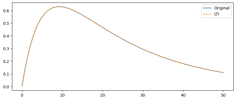
The synapse model was originally written as an explicit function of time since last spike. We know the expression represents a constant-coefficient LTI dynamical system with two state variables, we’ll solve its evolution over time and match parameters with the closed-form expression.
import numpy as np; import scipy
from matplotlib import pyplot as plt
tau_m=20; #membrane time constant
tau_s=5; #synaptic time rise epsp
eps0=20; #scaling constant epsp

t = np.linspace(0, 50, 500)
epsp = (eps0/(tau_m - tau_s))*(np.exp(-t/tau_m) - np.exp(-t/tau_s))

a = 1/tau_m
b = 1/tau_s
k = 1
dynmat = np.array([[-a, k],[0, -b]])
# Solution of above system is: x[0] = c1*exp(-at) + c2*k*(exp(-at) - exp(-bt))/(b - a); x[1] = c2*exp(bt)
# https://www.wolframalpha.com/input?i=solve+%28v%27%28t%29+%3D+kx+-av%2C++x%27%28t%29+%3D+-bx%29
# then epsp(0) = 0 => c1 = 0 and c2*k/(b-a) = e0/(tau_m - tau_s) => c2*k = e0*a*b
c = np.array([0,eps0*a*b])
eps0_corrected = eps0*a*b # to inject cells at the secondary state variable with
# Let's compare with the original solution
y = np.array([scipy.linalg.expm(dynmat * ti) @ c for ti in t])
plt.figure(figsize=[10,4]);
plt.plot(t, epsp); plt.plot(t,y[:,0], '--');
plt.legend(['Original','LTI']);
Let’s convert the models for the place and action cells from the original MATLAB code. Note that both the place cells and the action cells fire stochastically as a function of stimulation level:
## Action neurons - neuron model

# rho0=60*10**(-3); #scaling rate
# theta=16; #threshold
# delta_u=2; #escape noise
cell_defs = '''
<ComponentType name="DiscreteRandomishSpiker" extends="baseCell">
    <EventPort name="spike" direction="out"/>
    <Parameter name="rho_peak" dimension="per_time" description="Peak firing rate when mouse is right on the PC"/>
    <Parameter name="dt" dimension="time" description="Time step of the discrete update, TODO make more continuous and smooth"/>

    <Parameter name="pc_x" dimension="none" description="Horizontal component of this position cell's location"/>
    <Parameter name="pc_y" dimension="none" description="Vertical   component of this position cell's location"/>
    <Parameter name="pc_sigma" dimension="none" description="Spatial constant of this position cell's sensitivity"/>

    <VariableRequirement name="mouse_x" dimension="none" description="Horizontal component of agent's location"/>
    <VariableRequirement name="mouse_y" dimension="none" description="Vertical   component of agent's location"/>
    <Dynamics>
        <StateVariable name="lastUpdate" dimension="time"/>
        <DerivedVariable name="distance" dimension="none" value="sqrt((mouse_x-pc_x)^2+(mouse_y-pc_y)^2)" description="Distance of mouse from this PC"/>
        <DerivedVariable name="rho" dimension="per_time" value="rho_peak*exp(-((distance/pc_sigma)^2))"/>

        <OnCondition test="(1 == 1) .and. (random(1) .lt. (rho*dt))"><!-- TODO update explicitly and also stop when reward is reached -->
                    <EventOut port="spike"/>
            </OnCondition>
    </Dynamics>
</ComponentType>
<ComponentType name="SrmExpTwoCell" extends="baseCellMembPotCap"> <!-- not really cap but since baseSynapse exposes current... -->

    <Parameter name="v_rho_base" dimension="voltage" desc="Voltage midpoint for base spiking activity"/>
    <Parameter name="rho_base" dimension="per_time" desc="Scale of base spiking activity"/>
    <Parameter name="rho_scale" dimension="voltage" desc="Scale of exponential spiking activity growth"/>
    <Parameter name="dt" dimension="time" description="Time step of the discrete update, TODO make more continuous and smooth"/>

    <Parameter name="chi" dimension="voltage" description="Reset potential"/>
    <Parameter name="tau_m" dimension="time" description="Decay time constant for v"/>
    <Parameter name="tau_s" dimension="time" description="Decay time constant for I"/>
    <Parameter name="tau_gamma" dimension="time" description="Rise  time constant for rho"/>
    <Parameter name="v_gamma" dimension="time" description="Decay time constant for rho"/>
    <Constant name="msec" dimension="time" value="1 msec"/>

    <Dynamics>
            <StateVariable name="lastSpikeTime" dimension="time" exposure="lastSpikeTime"/>
        <StateVariable name="v" dimension="voltage" exposure="v"/>
        <StateVariable name="I" dimension="voltage" description="Exp decaying current stim, modelled as voltage bc this is a tau cell"/>
        <StateVariable name="spike_count" dimension="none"/>

        <StateVariable name="rho_decay" dimension="none"/> <!-- TODO express rho as one aggregate state variable and one latent -->
        <StateVariable name="rho_rise"  dimension="none"/>

        <DerivedVariable name="rho_tilda" dimension="per_time" value="rho_base*exp((v - v_rho_base)/rho_scale)" description="Instantaneous firing rate"/>

            <TimeDerivative variable="v" value="(-v / tau_m) + I/msec" />
            <TimeDerivative variable="I" value="(-I) / tau_s" />

            <TimeDerivative variable="rho_decay" value="-rho_decay / tau_gamma" />
            <TimeDerivative variable="rho_rise" value="-rho_rise / v_gamma" />
        <DerivedVariable name="rho_smooth" dimension="none" value="rho_decay-rho_rise" description="Smoothened firing rate"/>


        <OnStart> <!-- Start at resting state -->
            <StateAssignment variable="v" value="0*chi"/> <!-- TODO or zero? -->
            <StateAssignment variable="lastSpikeTime" value="t - tau_m*100" />
            <StateAssignment variable="spike_count" value="0" />
        </OnStart>

             <OnCondition test="(1 == 1) .and. (random(1) .lt. (rho_tilda*dt))"><!-- TODO stop when reward is reached -->
                    <EventOut port="spike"/>
            <StateAssignment variable="spike_count" value="spike_count+1" />
                    <StateAssignment variable="lastSpikeTime" value="t" /><!-- Refer to Canc in original code as to what gets reset-->
                    <StateAssignment variable="v" value="chi" />
                    <StateAssignment variable="I" value="0*I" />
            <StateAssignment variable="rho_decay" value="rho_decay + 1" />
            <StateAssignment variable="rho_rise"  value="rho_rise  + 1" />
            </OnCondition>
    </Dynamics>
</ComponentType>

<!-- NB: V_b may be overridden with EdenCustomSetup -->
<DiscreteRandomishSpiker id="PointCell" rho_peak="0.4 per_ms" dt="1 ms" pc_x="0" pc_y="0" pc_sigma="0.4" />
<SrmExpTwoCell id="ActionNeuron" dt="1 ms" v_rho_base="16 mV" rho_base="60 Hz" rho_scale="2 mV" chi="-5mV"
tau_m="20 ms" tau_s="5 ms" tau_gamma="50 ms" v_gamma="20 ms" C="0.2nF" />
'''
Note that some variables here like rho should be dimensional; figuring out the correct units for each parameter here is left as practice for the reader.
Let’s port the synapse models, plastic for input-to-output and static for lateral inhibition. Since the spike pathway is not covered by NeuroML for post-synapses and the firing mechanism is non-standard, we’ll have to detect spikes by adding spike counter to the cells and peeking into them (see also above for related additions).
## feed-forward synaptic plasticity parameters
ACh_flag=1; # cholinergic depression (1=+ACh; 0=-ACh)
eta_ACh = 1e-3*2; # learning rate acetylcholine

A_pre_post=1;   #amplitude pre-post window
A_post_pre=1;   #amplitude post-pre window
tau_pre_post= 10/2;   #time constant pre-post window. NOTE: altered from the original to correct for different numerical method.
tau_post_pre= 10;   #time constant post-pre window
tau_e= 2e3; #time constant eligibility trace

eta_DA=0.01; #learning rate eligibility trace HERE

w_max=3*1; #upper bound feed-forward weights
w_min=1; #lower bound feed-forward weights
syns_defs = f'''
<ComponentType name="ExpCurrLtiSyn" extends="baseSynapse"
    description="An exponential-current synapse with the quirk that current is modelled INSIDE the cell. TODO ">
    <Constant name="AMP" dimension="current" value="1 A"/>
    <Constant name="mV" dimension="voltage" value="1 mV"/>
    <Parameter name="wee" dimension="voltage" description="Weight really"/> <!-- TODO access the weight of the synapse  as defined on the projection, somehow -->
    <!-- <EventPort name="in" direction="in"/> -->
    <WritableRequirement name="I" dimension="voltage"/>
    <Dynamics>
            <DerivedVariable name="i" exposure="i" dimension="current" value="0 * AMP" />
            <OnEvent port="in">
                    <StateAssignment variable="I" value="I+wee*{eps0_corrected*1}" /> <!-- TODO dimension check! -->
            </OnEvent>
    </Dynamics>
</ComponentType> <!-- TODO updating., init weight, etc. -->
<ComponentType name="ExpCurrLtiSyn_Stdp" extends="baseSynapse"
    description="An exponential-current synapse with the quirk that current is modelled INSIDE the cell. TODO ">

    <Constant name="AMP" dimension="current" value="1 A"/>
    <Constant name="w_max" dimension="none" value="{w_max}"/>
    <Constant name="w_min" dimension="none" value="{w_min}"/>
    <Constant name="ACh_flag" dimension="none" value="{ACh_flag}"/>
    <Constant name="mV" dimension="voltage" value="1 mV"/> <!-- TODO access the weight of the synapse as defined on the projection, somehow -->

    <Parameter name="w_init" dimension="none"/>

    <Parameter name="A_pre_post" dimension="none"/>
    <Parameter name="A_post_pre" dimension="none"/>
    <Parameter name="tau_pre_post" dimension="time"/>
    <Parameter name="tau_post_pre" dimension="time"/>
    <Parameter name="tau_e" dimension="time"/>

    <Parameter name="eta_ACh" dimension="none"/>
    <Parameter name="eta_DA" dimension="none"/>

    <VariableRequirement name="current_trial" dimension="none"/>
    <VariableRequirement name="reward_found" dimension="none"/>
    <WritableRequirement name="I" dimension="voltage"/>
    <WritableRequirement name="spike_count" dimension="none"/> <!-- TODO this does not have to be Writable if Requirements can be resolved for the particular cell-synapse pairs (as done for WritableRequirement) -->
    <Dynamics>

        <StateVariable name="w"  dimension="none"/>
        <StateVariable name="e"  dimension="none"/>
        <StateVariable name="w_old"  dimension="none"/>
        <StateVariable name="conv_pre"  dimension="none"/>
        <StateVariable name="conv_post"  dimension="none"/>
        <StateVariable name="last_trial"  dimension="none"/>
        <StateVariable name="last_post_spike_count"  dimension="none"/>
        <StateVariable name="register_reward"  dimension="none"/>

            <DerivedVariable name="i" exposure="i" dimension="current" value="0 * AMP"/>
        <TimeDerivative variable="conv_pre"  value="-conv_pre /tau_pre_post"/>
        <TimeDerivative variable="conv_post" value="-conv_post/tau_post_pre"/>
        <TimeDerivative variable="e" value="-e/tau_e"/>

        <OnCondition test="w .lt. w_min"><StateAssignment variable="w" value="w_min"/></OnCondition>
        <OnCondition test="w .gt. w_max"><StateAssignment variable="w" value="w_max"/></OnCondition>
        <OnCondition test="(current_trial != last_trial)">
            <StateAssignment variable="w" value="w * (1-reward_found) + (w_old*eta_DA*e) * register_reward"/>

            <StateAssignment variable="conv_pre" value="0" />
            <StateAssignment variable="conv_post" value="0" />
            <StateAssignment variable="e" value="0" />

                    <StateAssignment variable="last_trial" value="current_trial" />
                    <StateAssignment variable="w_old" value="w" />

            <StateAssignment variable="register_reward" value="0"/>
        </OnCondition>

        <OnCondition test="reward_found > 0">
            <StateAssignment variable="register_reward" value="reward_found"/>
        </OnCondition>
        <OnCondition test="last_post_spike_count != spike_count">
            <StateAssignment variable="conv_post" value="conv_post+A_post_pre"/>
            <StateAssignment variable="e" value="e+conv_pre"/>
            <StateAssignment variable="w" value="w-eta_ACh*ACh_flag*conv_pre"/>
            <StateAssignment variable="last_post_spike_count" value="spike_count"/>
        </OnCondition>
            <OnEvent port="in">
                    <StateAssignment variable="I" value="I+w*{eps0_corrected*1}*mV"/>
                    <StateAssignment variable="conv_pre" value="conv_pre +A_pre_post"/>
            <StateAssignment variable="e" value="e+conv_post"/>
            <StateAssignment variable="w" value="w-eta_ACh*ACh_flag*conv_post"/>
            </OnEvent>
        <OnStart>
            <StateAssignment variable="w" value="w_init"/>
            <StateAssignment variable="last_trial" value="0"/>
            <StateAssignment variable="last_post_spike_count" value="0"/>
            <StateAssignment variable="register_reward" value="0"/>
        </OnStart>
    </Dynamics>
</ComponentType>
<ExpCurrLtiSyn id="LateralSynapse" wee="0 mV"/>
<ExpCurrLtiSyn_Stdp id="FeedforwardSynapse" w_init="2"
A_pre_post="{A_pre_post}" A_post_pre="{A_post_pre}"
tau_pre_post="{tau_pre_post} ms" tau_post_pre="{tau_post_pre} ms"
tau_e="{tau_e} ms" eta_ACh="{eta_ACh}" eta_DA="{eta_DA}"/>
'''
Let’s calculate the parameters which change among place cells, action cells, and connections thereof:
## Place cells
space_pc = 0.4 #place cells separation distance
bounds_x = [-2, +2] #bounds open field, x axis
bounds_y = [-2, +2] #bounds open field, y axis
x_pc = np.linspace(*bounds_x, int(np.diff(bounds_x)[0]/space_pc +1)) #place cells on axis x
n_x = len(x_pc); #nr of place cells on axis x
y_pc= np.linspace(*bounds_y, int(np.diff(bounds_y)[0]/space_pc +1))  #place cells on axis y
n_y = len(y_pc); #nr of place cells on axis y

#create grid of place cells
grid_x, grid_y = [z.ravel() for z in np.meshgrid(x_pc, y_pc)]
N_pc=len(grid_x); #number of place cells
## Action neurons - parameters
N_action=40; #number action neurons
theta_actor = 2*np.pi*np.arange(N_action)/N_action; #angles actions
action_dirs = np.array([np.sin(theta_actor), np.cos(theta_actor)]).T

#action selection
#winner-take-all weights
w_minus = -300;
w_plus = 100;

psi = 20; #the higher, the more narrow the range of excitation
diff_theta = np.tile(theta_actor, (N_action,1)) - np.tile(theta_actor, (N_action,1)).T
f = np.exp(psi*np.cos(diff_theta)); #lateral connectivity function
f -= np.diag(np.diag(f))
normalised = np.sum(f[0]) # NB all the rows/cols shoudl sum up to the same
w_lateral = (w_minus/N_action+w_plus*f/normalised); #lateral connectivity action neurons
# print(w_lateral[0])
lateral_conns =  [(i,j,w_lateral[i,j]) for i in range(N_action) for j in range(N_action)]
# TODO check if diag is ignored...
## delete actions that lead out of the maze
# find index place cells that lie on the walls
sides = [
    np.where(grid_y == bounds_y[0])[0], # bottom wall, y=-2
    np.where(grid_y == bounds_y[1])[0], # top    wall, y=+2
    np.where(grid_x == bounds_x[0])[0], # left   wall, x=-2
    np.where(grid_x == bounds_x[1])[0], # right  wall, x=+2
]
# store index of actions forbidden from each side with trig
ε = 1e-6 # for tolerance...
forbidden_actions = [
    np.where(action_dirs[:,1] < -ε)[0], # actions that point south - theta in (180, 360) degrees approx
    np.where(action_dirs[:,1] > +ε)[0], # actions that point north - theta in (  0, 180) degrees approx
    np.where(action_dirs[:,0] < -ε)[0] ,# actions that point eastt - theta in (-90,  90) degrees approx
    np.where(action_dirs[:,0] > +ε)[0], # actions that point westt - theta in ( 90, 270) degrees approx
]
# kill connections between place cells on the walls and forbidden actions
w_walls = np.ones([N_action, N_pc]);
for actt, sidd in zip(forbidden_actions, sides):
    for a in actt: w_walls[[a]*len(sidd), sidd] = 0

# show for debug
# plt.scatter(*action_dirs.T, s=0)#*range(N_action)) # for autoscale
# for i,(x,y) in enumerate(action_dirs):
#     txtt = ''.join([txt for actt, txt in zip(forbidden_actions, 'SNEW') if i in actt])
#     plt.text(x, y, f'{i}{txtt}', ha='center', va='center',c='r')
# print(w_walls[15].reshape([11,-1]), grid_y.reshape([11,-1]), sep='\n')

ff_conns = [(i,j) for i in range(N_pc) for j in range(N_action) if w_walls[j][i] > 0]
And let’s put it all together. We’ll expose one input stream and output stream to interact with the physical environment:
tabline = '\n    ' # annoyingly enough, \ may not exist at all in a f string, not even in brackets. Fixed in Python 3.12+

nml_file=f'''
<neuroml>

{cell_defs}
{syns_defs}

<!-- Here comes the network -->
<network id="Net">
    <!-- Add a population with a single cell -->
    <population id="PointCells" component="PointCell" size="{N_pc}"/>
    <population id="ActioCells" component="ActionNeuron" size="{N_action}"/>
    <projection id="Feedforward" presynapticPopulation="PointCells" postsynapticPopulation="ActioCells" synapse="FeedforwardSynapse">
        {tabline.join([ f'<connection id="{ii}" preCellId="{pre}" postCellId="{post}"/>' for ii, (pre,post) in enumerate(ff_conns)])}
    </projection>
    <projection id="Lateral" presynapticPopulation="ActioCells" postsynapticPopulation="ActioCells" synapse="LateralSynapse">
        {tabline.join([ f'<connection id="{ii}" preCellId="{pre}" postCellId="{post}"/>' for ii, (pre,post,w) in enumerate(lateral_conns)])}
    </projection>

    <!-- Add an input stream ❗ -->
    <EdenTimeSeriesReader id="Env"  href="file://EnvironmentToSnn.pipe" format="ascii_v0" instances="1" >
        <InputColumn id="mouse_x" dimension="none"/>
        <InputColumn id="mouse_y" dimension="none"/>
        <InputColumn id="trial_no" dimension="none"/>
        <InputColumn id="reward_found" dimension="none"/>
    </EdenTimeSeriesReader>
</network>
<Simulation id="MySim" length="200 s" step="1 ms" seed="9" target="Net"><!-- NOTE: leave the seed value unset to see varying behaviour -->
    <!--
    <EdenOutputFile id="ActioIntern" href="file://ac.gen.txt" format="ascii_v0" sampling_interval="1 msec">
        {tabline.join([ f'<OutputColumn id="v_{i}"  quantity="ActioCells[{i}]/v" output_units="mV"/>' for i in range(N_action)])}
        {tabline.join([ f'<OutputColumn id="I_{i}"  quantity="ActioCells[{i}]/I" output_units="mV"/>' for i in range(N_action)])}
    </EdenOutputFile>
    <EventOutputFile id="SpikesExc" fileName="spikes_pc.gen.txt" format="TIME_ID">
        {tabline.join([ f'<EventSelection id="{i}"  select="PointCells[{i}]" eventPort="spike"/>' for i in range(N_pc)])}
    </EventOutputFile>
    <EventOutputFile id="SpikesInh" fileName="spikes_ac.gen.txt" format="TIME_ID">
        {tabline.join([ f'<EventSelection id="{i}"  select="ActioCells[{i}]" eventPort="spike"/>' for i in range(N_action)])}
    </EventOutputFile>
    <EdenOutputFile id="Synnnn" href="file://synnnn.txt" format="ascii_v0" sampling_interval="1 msec">
        {tabline.join([ f'<OutputColumn id="decay_{i}"  quantity="Feedforward[{i}]/post/e"/>' for i, (pre,post) in enumerate(ff_conns) if pre==60 and post in list(range(1)) ])}
        {tabline.join([ f'<OutputColumn id="deca_{i}"  quantity="Feedforward[{i}]/post/conv_pre"/>' for i, (pre,post) in enumerate(ff_conns) if pre==60 and post in list(range(1)) ])}
        {tabline.join([ f'<OutputColumn id="decy_{i}"  quantity="Feedforward[{i}]/post/conv_post"/>' for i, (pre,post) in enumerate(ff_conns) if pre==60 and post in list(range(1)) ])}
    </EdenOutputFile>
     -->
    <EdenOutputFile id="MyOutSynsRec" href="file://actions.gen.txt" format="ascii_v0" sampling_interval="1 msec">
        {tabline.join([ f'<OutputColumn id="decay_{i}"  quantity="ActioCells[{i}]/rho_decay"/>' for i in range(N_action)])}
        {tabline.join([ f'<OutputColumn id="rise_{i}"  quantity="ActioCells[{i}]/rho_rise"/>' for i in range(N_action)])}
    </EdenOutputFile>
    <!-- Add an output stream ❗ -->
    <EdenOutputFile id="MyOutSyns" href="file://SnnToEnvironment.pipe" format="ascii_v0" sampling_interval="1 msec">
        {tabline.join([ f'<OutputColumn id="decay_{i}"  quantity="ActioCells[{i}]/rho_decay"/>' for i in range(N_action)])}
        {tabline.join([ f'<OutputColumn id="rise_{i}"  quantity="ActioCells[{i}]/rho_rise"/>' for i in range(N_action)])}
    </EdenOutputFile>

    <!-- Use EdenCustomSetup ❗ -->
    <EdenCustomSetup filename="CustomSetup.txt"/>
</Simulation>
<Target component="MySim"/></neuroml>
'''

# {tabline.join([ f'<OutputColumn id="v_{i}"  quantity= "Inh[{i}]/v"/>' for i in range(N_inh)])}
with open('Model.nml', 'wt') as f: f.write(nml_file)
eden_setup_lines = []
eden_setup_lines += ['set cell PointCells all all mouse_x Env[0]/mouse_x']
eden_setup_lines += ['set cell PointCells all all mouse_y Env[0]/mouse_y']
eden_setup_lines += ['set cell PointCells all all pc_x multi', 'values '+ ' '.join([str(w) for w in grid_x])]
eden_setup_lines += ['set cell PointCells all all pc_y multi', 'values '+ ' '.join([str(w) for w in grid_y])]
eden_setup_lines += ['set synapse Feedforward all post current_trial Env[0]/trial_no']
eden_setup_lines += ['set synapse Feedforward all post reward_found Env[0]/reward_found']
eden_setup_lines += ['set synapse Lateral all post wee multi mV', 'values '+ ' '.join([str(1*w) for (_,_,w) in lateral_conns])]
setup_file = '\n'.join(eden_setup_lines)
with open('CustomSetup.txt', 'wt') as f: f.write(setup_file)
import eden_simulator as eden
# tra, eve = eden.runEden('Model.nml', reload_events=True, threads=1)
Now let’s run the simulation with runEden … oh wait, we also need to simulate the environment! We’ll need a second process running in tandem, and Unix pipes or another conduit for exchanging streaming data. For debugging purposes, though, you can still use a normal file with place-holder trajectories.
%%writefile EnvironmentToSnn.pipe
0.0 0 0 1 0
Writing EnvironmentToSnn.pipe
# !eden nml Model.nml
Onward to writing the environment simulator: it needs to receive a stream of SNN output and provide a stream of input to the SNN. Watch out for deadlocks: each simulation must output trajectories covering at least one time step ahead of the data it received. One day the supporting machinery outside NewTrial and Advance may be provided by Eden for convenience.
%%writefile mechsim.py
#!/bin/python3
import sys; argv = sys.argv
import logging
logging.basicConfig(format='%(levelname)s:%(message)s', level=logging.DEBUG)
import numpy as np; import json

# parameters for the simulation
# else: raise ValueError(f'option "{type}" is not valid; only "event" or "trajectory" are')
input_from_snn_filename = argv[3] #'fifa'
output_to_snn_filename = argv[4] #'fifb'
output_log_filename = argv[5] if 6 <= len(argv) else 'mechsim.gen.txt'
output_report_filename = argv[6] if 7 <= len(argv) else 'mechmore.json'

# --- constants ---
TIME_STEP = 0.001
# TODO the roundoff can add a jitter of (sim dt) as it stands, make it work assuming dt is an integer timestep of usec...
delay = 0.002
## Task parameters
Trials = 40000; #number of trial TODO
T_max=15000; #maximum time trial
starting_position=[0,0]; #initialize position at origin (centre open field)
goals = [(+1.5,+1.5, 0.3), (-1.5,-1.5, 0.3)] # x, y, radius
dx = 0.01; #length of bouncing back from walls
bounds_x = [-2, +2] #bounds open field, x axis
bounds_y = [-2, +2] #bounds open field, y axis
N_action=40; #number action neurons
theta_actor = 2*np.pi*np.arange(N_action)/N_action; #angles actions
action_dirs = np.array([np.sin(theta_actor), np.cos(theta_actor)]).T
a0=.008/3; # actions = a0*action_dirs HERE

# logging.debug(f'ReadyA {type} {input_from_snn_filename} {output_to_snn_filename}')
# buffering is 0 to overcome 'not seekable' and binary is set bc can't have unbuffered *text* IO
# and write is not set because then the pipe would remain open (for this process that asked) forever
# Open the pipe for reading BEFORE the one for writing, because the latter can't be opened until the file has been opened for reading on the other side, likewise for the other process...
# or use async IO TODO

class MechSim:
    def __init__(self,**kwargs):
        self.fl = open(output_log_filename,'wt')
        self.InitModel(**kwargs)
    def InitModel(self,**kwargs):
        self.time = 0

        self.mechmore = {
            'time_goal':np.zeros([Trials, len(goals)]),
            'time_found':np.zeros([Trials, len(goals)]),
            'trial_started':[],
        }
        self.NewTrial(0)
        self.Log()
    def Sample(self):
        return [self.pos[0], self.pos[1], self.current_trial+1, self.reward_found]
    def Log(self):
        self.fl.write(f'{self.time} {self.pos[0]} {self.pos[1]} {self.current_trial} {self.reward_found} {self.current_action[0]} {self.current_action[1]} {self.current_motion[0]} {self.current_motion[1]}\n')
    def NewTrial(self, trial_no):
        if trial_no >= Trials: return
        # --- state ---
        self.current_trial = trial_no
        self.trial_started = self.time
        self.mechmore['trial_started'].append(self.trial_started)
        self.pos = np.array(starting_position) #position of the agent at each timestep
        self.current_action = [0,0]
        self.current_motion = [0,0]
        self.time_found = 0  # time of reward - initialized to 0 at the beginning of the trial
        self.reward_found = 0 # flag that signals when the reward is found
        self.current_goal = 0 if self.current_trial < 10 else 1 # TODO parameterise

    def Advance(self, newtime, numbers):
        advance_until = newtime + delay
        # print('adv', newtime, advance_until)
        action_smooth_decay = numbers[0:N_action]
        action_smooth_rise = numbers[N_action:N_action+N_action]
        action_smooth = np.array(action_smooth_decay) -  action_smooth_rise
        # select action
        self.current_action = a0*(action_dirs.T@action_smooth)/N_action
        # firing_rate_store(:,i) = rho_action_neurons; %store action neurons' firing rates
        for i,(x,y,r) in enumerate(goals):
            if np.linalg.norm(self.pos-[x,y]) <= r and self.mechmore['time_goal'][self.current_trial, i] == 0:
                self.mechmore['time_goal'][self.current_trial, i] = newtime
                if self.current_goal == i:
                    logging.debug(f'Success  : {newtime} {self.trial_started} {self.current_goal} {i}')
                    self.reward_found = 1
                    self.time_found = newtime
                    self.mechmore['time_found'][self.current_trial] = self.time_found

        ## position update
        self.current_motion = self.current_action
        max_delta = 0.01/5 # could also add a speed limiter here
        if np.linalg.norm(self.current_motion) > max_delta: self.current_motion *= max_delta/np.linalg.norm(self.current_motion)
        self.pos = self.pos+self.current_motion;
        # check if agent is out of boundaries. If it is, bounce back in the opposite direction
        if self.pos[0]<=bounds_x[0]: self.pos[0] = bounds_x[0]+dx
        if self.pos[1]<=bounds_y[0]: self.pos[1] = bounds_y[0]+dx
        if self.pos[0]>=bounds_x[1]: self.pos[0] = bounds_x[1]-dx
        if self.pos[1]>=bounds_y[1]: self.pos[1] = bounds_y[1]-dx

        # time when trial end is 300ms after reward is found
        ordd = self.trial_started + T_max/1000; shor=((self.time_found+.3) if self.time_found > 0 else np.inf)
        t_extreme = min(self.trial_started + T_max/1000, ((self.time_found+.3) if self.time_found > 0 else np.inf));
        if t_extreme < self.time:
            logging.debug(f'New trial: {t_extreme} {self.time} {self.current_trial} {i} {ordd} {shor} | {self.trial_started} {self.trial_started+2} {self.trial_started + T_max/1000} {T_max} {T_max/1000}')
            self.NewTrial(self.current_trial+1)

        while self.time < advance_until:
        #     world.Step(TIME_STEP, 10, 10)
            self.time += TIME_STEP
            self.Log()
        # self.Log()
        # print('adt', self.time, advance_until)
        # TODO out rate management? priority queue? a callback also?
        return
    def Fini(self):
        if self.fl: self.fl.close(); self.fl = None; print('Done!') # TODO leave some time to ensure this runs... are borken pipes always detected?
        with open(output_report_filename, 'wt') as f: json.dump({
            k:v.tolist() if isinstance(v, np.ndarray) else v for k,v in self.mechmore.items()},f)
sim = MechSim()
try:
    with open(input_from_snn_filename, 'r',buffering=1) as fi:
            logging.debug('ReadyA')
            with open(output_to_snn_filename, 'w',buffering=1) as fo:
                    logging.debug('ReadyA')
                    i = 0
                    spiking = False # TODO
                    # if spiking:
                    #       # logging.debug('waaaa!!')
                    #       fo.write(f'{delay}\n'.encode("utf-8"))
                    while fi:
                            s = fi.readline()
                            if not s:
                                    break
                            # when there is only the timestamp+'\n' it is not split... strip it and add \n
                            # or lstrip() + re.findall(r'^\S', st)[0] to preserve trailing whitespace
                            timestamp, sep, remainder = s.strip().partition(' ')
                            def SampSendOut():
                                    # Fetch a snapshot
                                    samp = sim.Sample()
                                    newstamp = sim.time
                                    # Make output
                                    outnums = samp

                                    # Send output
                                    newnums = ' '.join(map(str,outnums))
                                    upds = str(newstamp)+sep+newnums+'\n'#+f'A {i}! \n'
                                    # logging.debug(f'A {i} '+upds)
                                    fo.write(upds)

                            if not spiking and i == 0:
                                    SampSendOut() # we still need that first line for eden to begin. TODO a more elegant solution :/

                            # Parse input
                            timestamp = float(timestamp)
                            numbers = list(map(float,remainder.split()))
                            # Consume input
                            sim.Advance(timestamp, numbers)

                            SampSendOut()
                            i += 1
finally:
    sim.Fini()
Writing mechsim.py
Now let’s write a small script to launch both Eden and the custom environment simulator from the command line, and set up the pipes. This implementation works on Linux and maybe Mac, if you need it for Windows just ask. GNU parallel may also be convenient.
%%writefile doit.py
import os, subprocess
def EnlargeYourPipe(path): #
    # for truly huge sizes cut the pipe in two and install/run buffer(1) in between.
    fd = os.open(path, os.O_RDWR) # ideally flags should be 0x3 here for pure ioctl but i guess pipes don't like it
    try:
        import fcntl as fc
        # 1031 = F_SETPIPE_SZ but python3.11 doesn't provide it somehow
        ret = fc.fcntl(fd, 1031, 1024*1024) # LATER autodetect from /proc/sys/fs/pipe-max-size or just run windows
        # print(ret)
    finally:
        os.close(fd);fd = None
def any(iterable):
    for element in iterable:
        if element:
            return True
    return False
def run_with_pipes(cmdlines, fifo_pair_filenames):
    import subprocess; concurrent_processes = []
    try:
        for type, s_a, a_s in fifo_pair_filenames:
            # s_a, a_s = ( f'{runtime_dir}/'+x for x in (s_a, a_s))
            subprocess.call(['rm', s_a, a_s]);
            subprocess.call(['mkfifo', s_a, a_s]);
            for x in (s_a, a_s): EnlargeYourPipe(x)
            if s_a != a_s:
                p = subprocess.Popen(['python', 'mechsim.py', '0.010', type, f'{s_a}', f'{a_s}'])
                concurrent_processes.append(p)
        invocations = []
        for cmdline in cmdlines:
            p = subprocess.Popen(['bash', '-c', cmdline])
            invocations.append(p)
        for p in invocations:
            p.wait()
            if p.returncode:
                print('Retcode', p.returncode, 'for ',p.args)
        if any(p.returncode != 0 for p in invocations):
            print(435,[p.returncode for p in invocations])
            raise
    finally:
        for p in concurrent_processes:
            try:
                p.wait(timeout=.5) # give some time for graceful shutdown of aux processes
            except subprocess.TimeoutExpired: pass
        if any(p for p in concurrent_processes if p.returncode is None): print('Terminating remaining processes...')
        for p in (p for p in concurrent_processes if p.returncode is None):
            print(p)
            p.kill()
fifo_pair_filenames = [('trajectory', 'SnnToEnvironment.pipe','EnvironmentToSnn.pipe'),]; threads=1
cmdlines = [f'OMP_NUM_THREADS={threads} OMP_SCHEDULE=static eden nml Model.nml > log_eden.txt 2>&1']
run_with_pipes(cmdlines, fifo_pair_filenames)
Writing doit.py
And finally get the whole system running!
%%time
!python3 doit.py 2>simulation_log.txt
Done!
CPU times: user 537 ms, sys: 92.7 ms, total: 630 ms
Wall time: 36.3 s
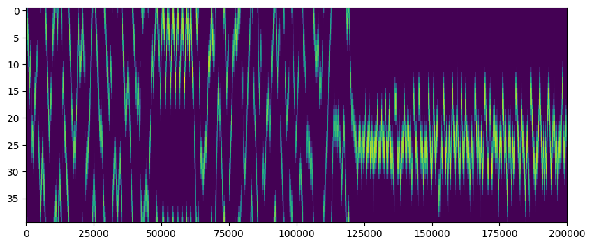
If all goes well, we can see how the output layer steered the agent. Thanks to lateral inhibition, only one direction is chosen at a time, and it changes smoothly. The membrane potential of the action cells can also prove useful to debug the layer’s behaviour, especially when comparing with the original.
neurdata = np.loadtxt('actions.gen.txt')
actions = neurdata[:,1:1+N_action] - neurdata[:,1+N_action:1+2*N_action] # Subtract rising from falling component
plt.figure(figsize=[10,4]);plt.imshow(actions.T,aspect='auto',interpolation='none');#plt.colorbar();
The environment simulator wrote down the state of the physical simulation over time (see Log(...) above). Let’s see what happened:
neurdata = np.loadtxt('mechsim.gen.txt')
labels = ['time', 'X loc.', 'Y loc.','Trial #','Reward','actx','acty','velx, vely']
plt.figure(figsize=[10,4]);plt.plot(neurdata[:,1:5],lw=1, label=labels[1:5]);plt.legend();
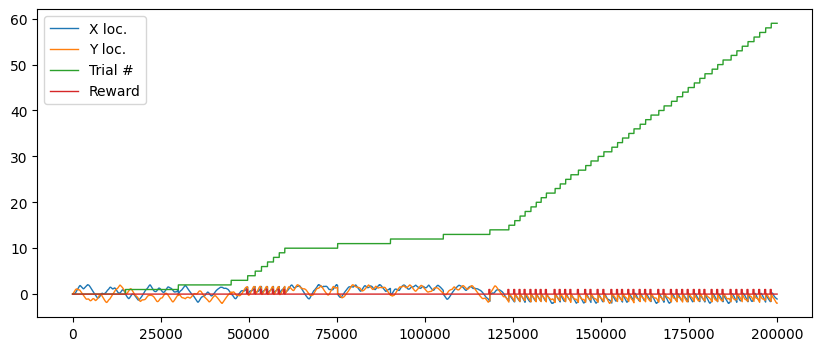
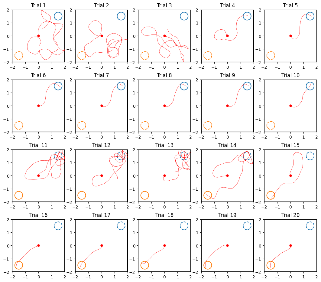
The trials add up over time, and as the SNN learns to navigate to the target they end faster in success. As per the original experiment, the reward is applied (and the new trial started) a short time after the target is reached.
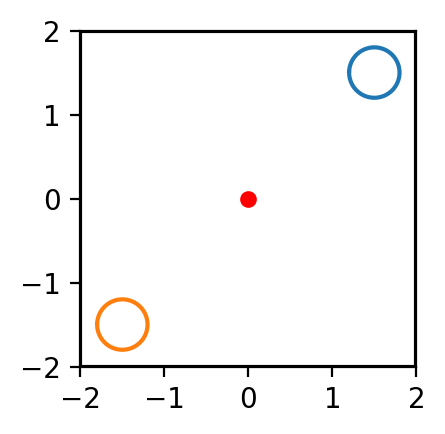
Let’s look at the AI agent’s trajectory within its confines (a trivial sort of labyrinth, if you think about it):
## plotting
starting_position=[0,0]; #initialize position at origin (centre open field)
goals = [(+1.5,+1.5, 0.3), (-1.5,-1.5, 0.3)] # x, y, radius
dx = 0.01; #length of bouncing back from walls
bounds_x = [-2, +2] #bounds open field, x axis
bounds_y = [-2, +2] #bounds open field, y axis
def PlotField(ax, mouse_traj=[], current_trial=None):
    # figure('position',  [0, 0, 1000, 2000])
    thetas = np.arange(-np.pi, +np.pi, 2*np.pi/100)

    for i,(x,y,r) in enumerate(goals): # plot goals
        current_goal = (i == (1 if current_trial > 9 else 0)) if current_trial is not None else True
        # print(f'{i}, {current_goal}')
        ax.plot(x+r*np.cos(thetas), y+r*np.sin(thetas), '-' if current_goal else '--')
    point_plot = ax.plot(*starting_position, '.r', ms=10); #plot initial starting point

    #plot walls
    ax.set_aspect('equal', 'box')
    ax.plot([bounds_x[0],bounds_x[0]], [bounds_y[0],bounds_y[1]],'k')
    ax.plot([bounds_x[1],bounds_x[1]], [bounds_y[0],bounds_y[1]],'k')
    ax.plot([bounds_x[0],bounds_x[1]], [bounds_y[0],bounds_y[0]],'k')
    ax.plot([bounds_x[0],bounds_x[1]], [bounds_y[1],bounds_y[1]],'k')
    ax.set_xlim(*bounds_x); ax.set_ylim(*bounds_y)

    #display trajectory of the agent in each trial
    if len(mouse_traj)>0: ax.plot(*mouse_traj, 'r',lw=.5);

    if current_trial is not None: ax.set_title(f'Trial {current_trial+1}')
plt.figure(dpi=200)
plt.subplot(2,2,1)
PlotField(plt.gca())
plt.figure();ax = plt.subplot(2,2,1)
PlotField(ax, neurdata[0:100000,1:3].T);
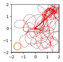
And trial by trial:
tracemax = len(neurdata)
on_reset       = np.all(neurdata[0:tracemax,1:3] == [0, 0], axis=1)
resets = np.r_[0,np.where(on_reset[1:] * ~on_reset[:-1])[0],tracemax]
# print(resets,len(resets))
plt.figure(figsize=[13,11.5])
for trial_no in range(20):#range(len(resets)-1):
    ax = plt.subplot(4,5,trial_no+1)
    PlotField(ax, neurdata[resets[trial_no]+1:resets[trial_no+1],1:3].T, trial_no);
plt.show()
# Or display them one by one:
# for trial_no in range(len(resets)-1):
#     plt.figure();ax = plt.subplot(2,2,1)
#     PlotField(ax, neurdata[resets[trial_no]+1:resets[trial_no+1],1:3].T, trial_no);
#     plt.show()
Feel free to draw the separate trials as progressive shades on the same environment, and animate the evolving policy as a vector field of Σ (action weights * action direction) per place cell.